Question 10.9.1: Consider the P, PI, and modified I control systems discussed......
Consider the P, PI, and modified I control systems discussed in Examples 10.6.2, 10.6.3, and 10.6.4. The plant transfer function is 1/(I s+c), where I = 5 and c = 2. This plant can represent an inertia whose rotational velocity is the output and whose input is a torque. So the control systems are examples of speed controllers.
Investigate the performance of these systems for the trapezoidal command input shown in Figure 10.9.1. Use the parameter values I = 5 and c = 2.

Learn more on how do we answer questions.
The transfer functions and parameters for these three control systems are shown in Table 10.9.1.
We can use the expressions in Table 10.9.1 to compute the gain values required to achieve a time constant of τ = 1 and a steady-state error e_{ss} = 0.2 for a unit-ramp command. Because the slope of the profile is 10/3, this will give a steady-state error of 0.2(10/3) = 2/3. The following table shows the results.
The following file sets the gain values for the three systems. System a is the P control system, system b is the PI system, and system c is the modified I system.
| — | K_P = 3 | P |
| K_I = 10 | K_P = 8 | PI |
| K_I = 50 | K_2 = 8 | Modified I |
Table 10.9.1 P, PI, and modified I control systems.
| Reference: Examples 10.6.2, 10.6.3, and 10.6.4 | |||
| Modified I | PI | P | |
| \frac{K_I}{5 s^2+\left(2+K_2\right) s+K_I} | \frac{K_P s + K_I}{5 s^2 + \left(2 + K_P\right) s + K_I} | \frac{K_P}{5 s + 2 + K_P} | Command transfer function Ω(s)/Ω_r (s) |
| -\frac{s}{5 s^2 + \left(2 + K_2\right) s + K_I} | -\frac{s}{5 s^2 + \left(2 + K_P\right) s + K_I} | -\frac{1}{5 s + 2 + K_P} | Disturbance transfer function Ω(s)/T_d (s) |
| \frac{(5 s + 2) K_I}{5 s^2 + \left(2 + K_2\right) s + K_I} | \frac{\left(K_P s + K_I\right)(5 s + 2)}{5 s^2 + \left(2 + K_P\right) s + K_I} | K_P \frac{5 s + 2}{5 s + 2 + K_P} | Actuator transfer function T (s)/T_d (s) |
| \frac{2 + K_2}{K_I} | \frac{2}{K_I} | \frac{1}{2 + K_P} | Steady-state unit-ramp error e_{ss} |
| \frac{10}{2 + K_2} \quad \text { if } \zeta \leq 1 | \frac{10}{2 + K_P} \quad \text { if } \zeta \leq 1 | \frac{5}{2 + K_P} | Time constant τ |
| \frac{2 + K_2}{2 \sqrt{5 K_I}} | \frac{2 + K_P}{2 \sqrt{5 K_I}} | — | Damping ratio ζ |
Table 10.9.2 Transfer function files.
| % command_tf.m % Create the command transfer functions. sysa = tf(KPa,[5, 2+KPa]); sysb = tf([KPb, KIb],[5, 2+KPb, KIb]); sysc = tf(KIc,[5, 2+K2, KIc]); |
| % actuator_tf.m % Create the actuator transfer functions. sysaACT = tf(KPa*[5, 2],[5, 2+KPa]); sysbACT = tf(conv([KPb, KIb],[5, 2]),[5, 2+KPb, KIb]); syscACT = tf(KIc*[5, 2],[5, 2+K2, KIc]); |
| % dist_tf.m % Create the disturbance transfer functions. sysaDIS = tf(-1, [5, 2+KPa]); sysbDIS = tf(-[1, 0],[5, 2+KPb, KIb]); syscDIS = tf(-[1, 0],[5, 2+K2, KIc]); |
Table 10.9.3 Solution and plotting files.
| % plot_command.m % Obtain and plot the command response. ya = lsim(sysa,r,t); yb = lsim(sysb,r,t); yc = lsim(sysc,r,t); plot(t,ya,t,yb,t,yc,’–‘,t,r) |
| % plot_actuator.m % Obtain and plot the actuator repsonse. yaACT = lsim(sysaACT,r,t); ybACT = lsim(sysbACT,r,t); ycACT = lsim(syscACT,r,t); plot(t,yaACT,t,ybACT,t,ycACT,’- -‘) |
| % plot_dist.m % Add the disturbance response to the command response % and plot the total response. ya = lsim(sysa,r,t); yb = lsim(sysb,r,t); yc = lsim(sysc,r,t); disturbance = 20*t; yaDIS = lsim(sysaDIS,disturbance,t); ybDIS = lsim(sysbDIS,disturbance,t); ycDIS = lsim(syscDIS,disturbance,t); plot(t,ya+yaDIS,t,yb+ybDIS,t,yc+ycDIS,’- -‘,t,r) |
Learn more on how do we answer questions.
Script File
% gains.m
% Sets the gains.
% P control (system a):
KPa = 3;
% PI control (system b):
KPb = 8 ; KIb = 10;
% I action modified with velocity feedback (system c):
K2 = 8 ; KIc = 50;
After running the program \boxed{gains.m}, the files shown in Table 10.9.2 are used to create the command, disturbance, and actuator transfer functions given in Table 10.9.1.
The trapezoidal command input shown in Figure 10.9.1 can be created with the following script file.
% trap.m
% A specific trapezoidal profile
t = (0:0.01:12);
for k = 1:length(t)
if t(k) <= 3
r(k) = (10/3)*t(k);
elseif t(k) <= 6
r(k) = 10;
elseif t(k) <= 9
r(k) = 30-(10/3)*t(k);
else
r(k) = 0;
end
end
After running \boxed{trap.m} and one of the transfer function programs given in Table 10.9.2, the files shown in Table 10.9.3 are used to compute and plot the command, disturbance, and actuator responses.
For example, to create the plot shown in Figure 10.9.2, use the M-file:
gains
command_tf
trap
plot_command
Notice that the P control system does not follow the trapezoidal profile very well. (Figure 10.9.2 was enhanced using the Plot Editor.)
The performance of the P control system can be improved by increasing the gain. For example, to use K_P = 50, change \boxed{KPa} to 50 in \boxed{gains.m} and run the following M-file. Note that we need not run \boxed{trap.m} again unless we cleared the variables.
gains
command_tf
plot_command
The result is shown in Figure 10.9.3. Now the P control follows the trapezoidal profile much better.
The actuator response is found by running the M-file:
actuator_tf
plot_actuator
The result is shown in Figure 10.9.4.
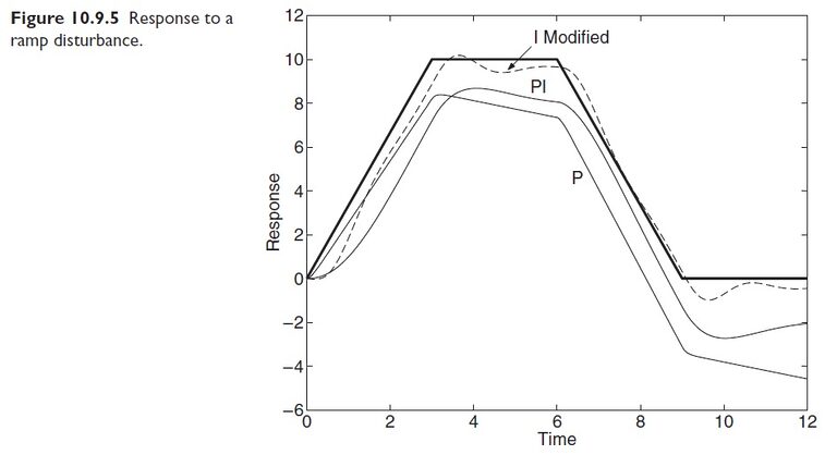
Finally, let us see how well the systems do with a ramp disturbance T_d = 20t. Run the following M-file.
dist_tf
plot_dist
The total response is shown in Figure 10.9.5. Both PI and P control have difficulty following the profile, but the modified I system does rather well.