Question 4.5: Comparison of Flow Patterns in an Unsteady Flow An unsteady,...
Comparison of Flow Patterns in an Unsteady Flow
An unsteady, incompressible, two-dimensional velocity field is given by
\vec{V} = (u , \upsilon ) = (0.5 + 0.8x)\vec{i} + (1.5 + 2.5 \sin (\omega t) – 0.8y)\vec{j} (1)
where the angular frequency 𝜔 is equal to 2𝜋 rad/s (a physical frequency of 1 Hz). This velocity field is identical to that of Eq. 1 of Example 4–1 except for the additional periodic term in the 𝜐-component of velocity. In fact, since the period of oscillation is 1 s, when time t is any integral multiple of \frac{1}{2} s (t = 0, \frac{1}{2} , 1, \frac{3}{2} , 2, . . . s), the sine term in Eq. 1 is zero and the velocity field is instantaneously identical to that of Example 4–1. Physically, we imagine flow into a large bell mouth inlet that is oscillating up and down at a frequency of 1 Hz. Consider two complete cycles of flow from t = 0 s to t = 2 s. Compare instantaneous streamlines at t = 2 s to pathlines and streaklines generated during the time period from t = 0 s to t = 2 s.
Learn more on how we answer questions.
Streamlines, pathlines, and streaklines are to be generated and compared for the given unsteady velocity field.
Assumptions 1 The flow is incompressible. 2 The flow is two-dimensional, implying no z-component of velocity and no variation of u or 𝜐 with z.
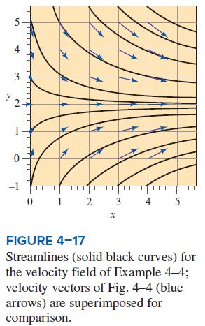
Analysis The instantaneous streamlines at t = 2 s are identical to those of Fig. 4–17, and several of them are replotted in Fig. 4–27. To simulate pathlines, we use the Runge–Kutta numerical integration technique to march in time from t = 0 s to t = 2 s, tracing the path of fluid particles released at three locations: (x = 0.5 m, y = 0.5 m), (x = 0.5 m, y = 2.5 m), and (x = 0.5 m, y = 4.5 m).
These pathlines are shown in Fig. 4–27, along with the streamlines. Finally, streaklines are simulated by following the paths of many fluid tracer particles released at the given three locations at times between t = 0 s and t = 2 s, and connecting the locus of their positions at t = 2 s. These streaklines are also plotted
in Fig. 4–27.
Discussion Since the flow is unsteady, the streamlines, pathlines, and streaklines are not coincident. In fact, they differ significantly from each other. Note that the streaklines and pathlines are wavy due to the undulating 𝜐-component of velocity. Two complete periods of oscillation have occurred between t = 0 s and t = 2 s, as verified by a careful look at the pathlines and streaklines. The streamlines have no such waviness since they have no time history; they represent an instantaneous snapshot of the velocity field at t = 2 s.