Question 2.2: The calculations using symmetrical components can best be il......
The calculations using symmetrical components can best be illustrated with an example. Consider a subtransmission system as shown in Figure 2.9. A 13.8 kV generator G_{1} voltage is stepped up to 138 kV. At the consumer end the voltage is stepped down to 13.8 kV, and generator G_{2} operates in synchronism with the supply system. Bus B has a 10,000 hp motor load. A line-to-ground fault occurs at bus B. It is required to calculate the fault current distribution throughout the system and also the fault voltages. The resistance of the system components is ignored in the calculations.

Learn more on how do we answer questions.
Impedance Data
The impedance data for the system components are shown in Table 2.2. Generators G_{1} and G_{2} are shown solidly grounded, which will not be the case in a practical installation.
A high-impedance grounding system is used by utilities for grounding generators in step-up transformer configurations. Generators in industrial facilities, directly connected to the load buses, are low-resistance grounded, and the ground fault currents are limited to 200–400 A. The simplifying assumptions in the example are not applicable to a practical installation, but clearly illustrate the procedure of calculations.
The first step is to examine the given impedance data. Generator-saturated subtransient reactance is used in the short-circuit calculations and this is termed positive sequence reactance; 138 kV transmission line reactance is calculated from the given data for conductor size and equivalent conductor spacing. The zero sequence impedance of the transmission line cannot be completely calculated from the given data and is estimated on the basis of certain assumptions, that is, a soil resistivity of 100 Ω-m.
Compiling the impedance data for the system under study from the given parameters, from manufacturers’ data, or by calculation and estimation can be time consuming. Most computer-based analysis programs have extensive data libraries and companion programs for calculation of system impedance data and line constants, which has partially removed the onus of generating the data from step-by-step analytical calculations. Appendix B provides models of line constants for coupled transmission lines, bundle conductors, and line capacitances. Refs. [3,4] provide analytical and tabulated data.
Next, the impedance data are converted to a common MVA base. A familiarity with the per unit system is assumed. The voltage transformation ratio of transformer T_{2} is 138–13.2 kV, while a bus voltage of 13.8 kV is specified, which should be considered in transforming impedance data on a common MVA base. Table 2.2 shows raw impedance data and their conversion into sequence impedances.
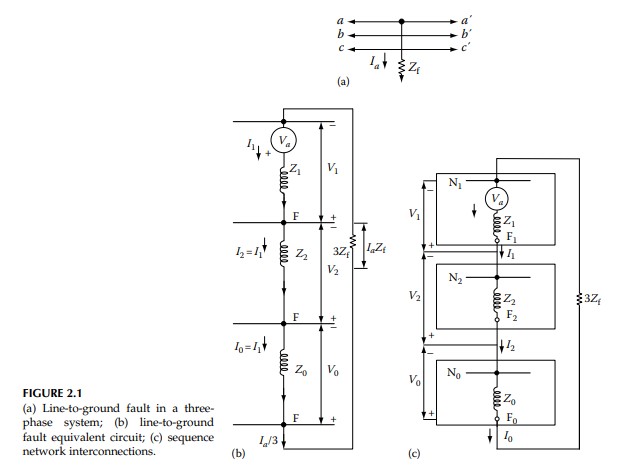
For a single line-to-ground fault at bus B, the sequence impedance network connections are shown in Figure 2.10, with the impedance data for components clearly marked. This figure is based on the fault equivalent circuit shown in Figure 2.1b, with fault impedance Z_{f} = 0. The calculation is carried out in per unit, and the units are not stated in every step of the calculation.
The positive sequence impedance to the fault point is
This gives Z_{1} = j0.212.
Z_{2}=\frac{j(0.28 \ + \ 0.18 \ + \ 0.04 \ + \ 0.24) \ × \ \frac{j0.55 \ × \ j1.8}{j(0.55 \ + \ 1.8)}}{j(0.28 \ + \ 0.18 \ + \ 0.04 \ + \ 0.24) \ + \ \frac{j0.55 \ × \ j1.8}{j(0.55 \ + \ 1.8)}}This gives Z_{2} = j0.266.
Z_{0} = j0.2. Therefore,
I_{1}= \frac{E}{Z_{1} \ + \ Z_{2} \ + \ Z_{0}}=\frac{1}{j0.212 \ + \ j0.266 \ + \ j0.2}=-j1.45 \ pu
I_{2}=I_{0}=-j1.475
I_{a} = I_{0} + I_{1} + I_{2} = 3(-j1.475) = -j4.425 \ pu
In terms of actual values this is equivalent to 1.851 kA. The fault currents in phases b and c are zero:
I_{b} = I_{c} = 0
The sequence voltages at a fault point can now be calculated:
V_{0} = -I_{0}Z_{0} = j1.475 × j0.2 = -0.295
V_{2} = -I_{2}Z_{2} = j1.475 × j0.266 = -0.392
V_{1} = E – I_{1}Z_{1} = I_{1}(Z_{0} + Z_{2}) = 1 – (-j1.475 × j0.212) = 0.687
A check of the calculation can be made at this stage; the voltage of the faulted phase at fault point B = 0:
V_{a} = V_{0} + V_{1} + V_{2} = -0.295 – 0.392 + 0.687 = 0
The voltages of phases b and c at the fault point are
V_{b} = V_{0} + aV_{1} + a^2 V_{2}
= V_{0} – 0.5(V_{1} + V_{2}) – j0.866(V_{1} – V_{2})
= -0.295 – 0.5(0.687 – 0.392) – j0.866(0.687 + 0.392)
= -0.4425 – j0.9344
|V_{b}| = 1.034 pu
Similarly,
V_{c} = V_{0} – 0.5(V_{1} + V_{2}) + j0.866(V_{1} – V_{2})
= -0.4425 + j0.9344
|V_{c}| = 1.034 pu
The distribution of the sequence currents in the network is calculated from the known sequence impedances. The positive sequence current contributed from the right side of the fault, that is, by G_{2} and motor M is
This gives -j1.0338. This current is composed of two components, one from the generator G_{2} and the other from the motor M. The generator component is
(-j1.0338) \frac{j1.67}{j(0.37 \ + \ 1.67)}=-j0.8463The motor component is similarly calculated and is equal to -j0.1875.
The positive sequence current from the left side of bus B is
This gives -j0.441. The currents from the right side and the left side should sum to -j1.475. This checks the calculation accuracy.
The negative sequence currents are calculated likewise and are as follows:
In generator G_{2} = -j0.7172
In motor M = -j0.2191
From left side, bus B = -j0.5387
From right side = -j0.9363
The results are shown in Figure 2.10. Again, verify that the vectorial summation at the junctions confirms the accuracy of calculations.
Currents in Generator G_{2}
I_{a}(G_{2}) = I_{1}(G_{2}) + I_{2}(G_{2}) + I_{0}(G_{2})
= -j0.8463 – j0.7172 – j1.475
= -j3.0385
|I_{a}(G_{2})| = 3.0385 pu
I_{b}(G_{2}) =I_{0} – 0.5(I_{1} + I_{2}) – j0.866(I_{1} – I_{2})
= -j1.475 – 0.5(-j0.8463 – j0.7172) – j0.866(-j0.8463 + j0.7172)
= -0.1118 – j0.6933
|I_{b} (G_{2})| = 0.7023 pu
I_{c}(G_{2}) = I_{0} – 0.5(I_{1} + I_{2}) + j0.866(I_{1} – I_{2})
= 0.1118 – j0.6933
| I_{c}(G_{2})| = 0.7023 pu
This large unbalance is noteworthy. It gives rise to increased thermal effects due to negative sequence currents and results in overheating of the generator rotor. A generator will trip quickly on negative sequence currents.
Currents in Motor M
The zero sequence current in the motor is zero, as the motor wye-connected windings are not grounded as per industrial practice in the United States. Thus,
I_{a}(M) = I_{1}(M) + I_{2}(M)
= -j0.1875 – j0.2191
= -j0.4066
|I_{a}(M)| = 0.4066 pu
I_{b}(M) = -0.5(-j0.4066) – j0.866(0.0316) = 0.0274 + j0.2033
I_{c}(M) = -0.0274 + j0.2033
|I_{b} (M)| = |I_{c}(M)| = 0.2051 pu
The summation of the line currents in the motor M and generator G_{2} are
I_{a}(G_{2}) + I_{a}(M) = -j3.0385 – j0.4066 = -j3.4451
I_{b}(G_{2}) + I_{b}(M) = -0.118 – j0.6993 + 0.0274 + j0.2033 = -0.084 – j0.490
I_{c}(G_{2}) + I_{c}(M) = 0.1118 – j0.6933 – 0.0274 + j0.2033 = 0.084 – j0.490
Currents from the left side of the bus B are
I_{a} = -j0.441 – j0.5387
= -j0.98
I_{b} = -0.5(-0.441 – j0.5387) – j0.866(-0.441 + j0.5387)
= 0.084 + j0.490
I_{c} = -0.084 + j0.490
These results are consistent as the sum of currents in phases b and c at the fault point from the right and left side is zero and the summation of phase a currents gives the total ground fault current at b = -j4.425. The distribution of currents is shown in a three-line diagram (Figure 2.11).
Continuing with the example, the currents and voltages in the transformer T_{2} windings are calculated. We should correctly apply the phase shifts for positive and negative sequence components when passing from delta secondary to wye primary of the transformer. The positive and negative sequence current on the wye side of transformer T_{2} are
I_{1( p)} = I_{1} < 30° = -j0.441 < 30° = 0.2205 – j0.382
I_{2( p)} = I_{2} < -30° = -j0.5387 < -30° = -0.2695 – j0.4668
Also, the zero sequence current is zero. The primary currents are
I_{a( p)} = I_{1( p)} + I_{2( p)}
= 0.441 < 30° + 0.5387 < -30° = -0.049 – j0.8487
I_{b( p)} = a^2 I_{1( p)} + aI_{2( p)} = -0.0979
I_{c( p)} = aI_{1( p)} + a^2 I_{2( p)} = -0.049 – j0.8487
Currents in the lines on the delta side of the transformer T_{1} are similarly calculated. The positive sequence component, which underwent a 30° positive shift from delta to wye in transformer T_{2}, undergoes a -30° phase shift; as for an ANSI connected transformer it is the low-voltage vectors, which lag the high-voltage side vectors. Similarly, the negative sequence component undergoes a positive phase shift. The currents on the delta side of
transformers T_{1} and T_{2} are identical in amplitude and phase. Note that 138 kV line is considered lossless. Figure 2.11 shows the distribution of currents throughout the distribution system.
The voltage on the primary side of transformer T_{2} can be calculated. The voltages undergo the same phase shifts as the currents. Positive sequence voltage is the base fault positive sequence voltage, phase shifted by 30° (positive) minus the voltage drop in transformer reactance due to the positive sequence current:
V_{1}( p) = 1.0 < 30° – jI_{1( p)}X_{2}
= 1.0 < 30° – ( j0.441 < 30°)( j0.24)
= 0.9577 + j0.553
V_{2}( p) = 0 – I_{2( p)}X_{2}
= -(0.539 < -30°)( j0.24)
= 0.112 – j0.0647
Thus,
V_{a( p)} = 0.9577 + j0.553 + 0.112 – j0.0647 = 1.0697 + j0.4883 = 1.17 < 24.5°
V_{b( p)} = -0.5(V_{1( p)} + V_{2( p)}) – j0.866(V_{1( p)} – V_{2( p)})
= -j0.9763
V_{c( p)} = 0.5(V_{1( p)} + V_{2( p)}) – j0.866(V_{2( p)} – V_{1( p)})
= 1.0697 + j0.4883 = 1:17 < 155.5°
Note the voltage unbalance caused by the fault.
| TABLE 2.2 Impedance Data for Example 2.2 |
||||
| Equipment | Description | Impedance Data | Per Unit Impedance 100 MVA Base | |
| G_{1} | 13.8 kV, 60 MVA, 0.85 power factor generator | Subtransient reactance = 15% Transient reactance = 20% Zero sequence reactance = 8% Negative sequence reactance = 16.8% |
X_{1} = 0.25 X_{2} = 0.28 X_{0} = 0.133 |
|
| T_{1} | 13.8–138 kV step-up transformer, 50=84 MVA, delta–wye-connected, wye neutral solidly grounded |
Z = 9% on 50 MVA base | X_{1}=X_{2}=X_{0} = 0.18 | |
| L_{1} | Transmission line, 5 mi. long, 266.8 KCMIL, ACSR | Conductors at 15 ft (4.57 m) equivalent spacing |
X_{1}=X_{2} = 0.04 X_{0}=0.15 |
|
| T_{2} | 138–13.2 kV, 30 MVA step-down transformer, wye–delta- connected, high-voltage wye neutral solidly grounded |
Z = 8% | X_{1}=X_{2}=X_{0} = 0.24 | |
| G_{2} | 13.8 kV, 30 MVA, 0.85 power factor generator | Subtransient reactance = 11% Transient reactance = 15% Zero sequence reactance = 6% Negative sequence reactance = 16.5% |
X_{1} = 0.37 X_{2} = 0.55 |
|
| M | 10,000 hp induction motor load | Locked rotor reactance = 16.7% on motor base kVA (consider 1 hp ≈ 1 kVA) |
X_{0} = 0.20 X_{1} = 1.67 |
|
| X_{2} = 1.80 X_{0}= \infty |
||||
Resistances are neglected in the calculations. KCMIL: Kilo-circular mils, same as MCM. ACSR: Aluminum conductor steel reinforced.