Question 19.3.b: DRIVING DISTANCES FOR GOLF BALL BRANDS (CONTINUED) One golf ......

Let μ_{C,W} be the mean yardage for brand C balls hit in warm weather, and define similar means for the other brands and temperatures. Then the first claim concerns the contrast

μ_{C,C}-\frac{μ_{A,C}+μ_{B,C}+μ_{D,C}+μ_{E,C}}{4}

and the second concerns the contrast

\frac{μ_{E,M}+μ_{E,W}}{2}-\frac{\frac{μ_{A,M}+μ_{A,W}}{2}+\frac{μ_{B,M}+μ_{B,W}}{2}+\frac{μ_{C,M}+μ_{C,W}}{2}+\frac{μ_{D,M}+μ_{D,W}}{2}}{4}\\[0.4cm] = \frac{μ_{E,M}+μ_{E,W}}{2} – \frac{μ_{A,M}+μ_{A,W}+μ_{B,M}+μ_{B,W}+μ_{C,M}+μ_{C,W}+μ_{DA,M}+μ_{D,W}}{8}

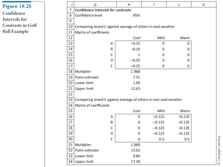
(Note in this second contrast how we average over the mild and warm temperatures. This is because the second claim just specifies “not cool.”) A good way to handle the calculations in Excel is illustrated in Figure 19.25. For either contrast, you first record the coefficients of the means in the contrast. These appear in the ranges H13:J17 and H26:J30. (Note that the sum of the values in each of these ranges is 0. This is required for contrasts, as we discussed previously.) Then the point estimate of a contrast is the SUMPRODUCT of the sample means and these coefficients. For example, you calculate the point estimate of the first contrast in cell H19 with the formula

=SUMPRODUCT(H13:J17,B19:D23)

The multiplier for these confidence intervals is always a thorny issue, but most statisticians agree that if only a small number of confidence intervals are being formed, as in this example, then you can use the usual t-value, where the degrees of freedom is the one corresponding to the error (within) variation. Therefore, the multiplier for each contrast is approximately 2, found in cell H18 with the formula

=TINV(1-H8,C40)

Then because each sample size is 20 (the value in cell B9), you can find the lower and upper limits of the confidence intervals from Expression (19.5). For example, the confidence interval for the first contrast is found with the formulas

=H19-H18*SQRT(D40*SUMSQ(H13:J17)/B9)

and

=H19+H18*SQRT(D40*SUMSQ(H13:J17)/B9)

in cells H20 and H21.

Confidence Interval for Contrast

Point estimate of contrast ± multiplier × \sqrt{\text{MSW}\sum\limits_{j}{c^2_j/n_j} }       (19.5)

As you can see, both claims are supported. The confidence intervals for the two contrasts extend from 1.99 to 12.63 and from 9.86 to 17.38—all positive yardages. It looks like brand C beats the average of the competition by at least 1.99 yards in cool weather, and brand E beats the average of the competition by at least 9.86 yards in weather that is not cool.