Question 19.5: THE EFFECT OF SOAP DISPENSERS ON SOAP SALES SoftSoap Company......

At first glance, this might look exactly like a one-way design as described in Section 19-2. There is a single factor, dispenser type, varied at four levels, and there are eight observations at each level. For example, we obtain a count of sales for dispenser type 1 at each of eight stores. However, it is very possible that the dependent variable, number of sales, is correlated with store. That is, some stores might sell a lot of each dispenser type, whereas others might not sell many of any dispenser type. (For example, stores in areas where there are a lot of manual labor jobs might sell a lot more hand soap than stores in a university area.) Therefore, we treat each store as a block, so that the experimental design appears as in Figures 19.30 and 19.31. Each treatment level (dispenser type) is assigned exactly once to each block (store). As a practical matter, if each dispenser type is stocked on a different shelf in the store, randomization could also be used, where each store is instructed to randomize the order of dispenser types from top shelf to bottom shelf.

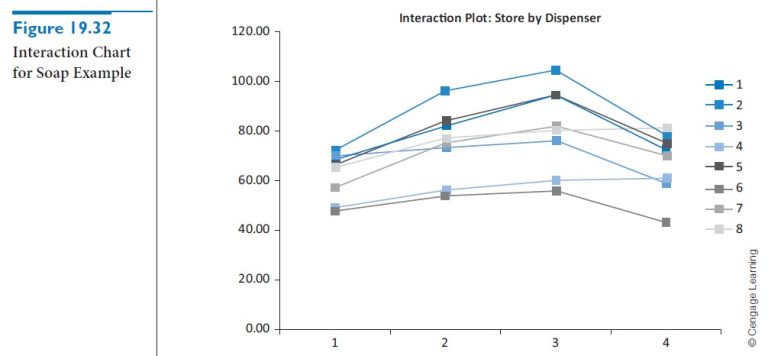
You can analyze these data essentially the same way you analyze a two-factor design, that is, with two-way ANOVA. There are two differences, one technical and one of inter-pretation. The technical difference is that because there is only one observation in each combination of treatment level and block, it is impossible to estimate an interaction effect and a “within” error variance simultaneously. Therefore, we assume there are no important interaction effects between treatment levels and blocks, and we attribute all variation other than that from main effects to error variation. The output is shown in Figure 19.31. To obtain this output, use the StatTools Two-Way ANOVA procedure, with Store and Dispenser as the two categorical variables. Because there is only one observation per store/dispenser combination, the ANOVA table has no Interaction row. Nevertheless, it still provides interaction charts, one of which appears in Figure 19.32, to check for the no-interaction assumption. If there were no interactions, the lines in this chart (one for each store) would be parallel. Although these lines are not exactly parallel, it appears that the effect of dispenser type is approximately the same at each store. Therefore, the no-interaction assumption appears justified.

There are two F-values and corresponding p-values in the ANOVA table in Figure 19.31. The one in row 47 is for the main effect of dispenser type, whereas the one in row 46 is for the main effect of store. The former is of more interest because this is the focus of the experiment. Its p-value is essentially 0, meaning that there are significant differences across dispenser types. In fact, judging by the sample means, the ranking of dispenser types in decreasing order is 3, 2, 4, 1, and there is a considerable gap between each of these. If SoftSoap had to market only one dispenser type, it would almost certainly select type 3. The p-value for the main effect of store is also essentially 0, which means that the stores differ significantly with respect to average sales. This is not as interesting a finding—in fact, we use a block design precisely because we suspect such an effect—but it does confirm that a block design is a good idea.

We can also confirm that blocking was useful by running a one-way ANOVA on the data, using Dispenser as the single factor and ignoring Store. The results appear in Figure 19.33. The differences across dispenser type are still significant at the 5% level (the p-value is still less than 0.05), but they are not as significant as when a blocking variable is used. By comparing the ANOVA tables in Figures 19.31 and 19.33, you can see that the error (within) sum of squares in the latter, 5042.5, is split into two parts in the former: the block sum of squares, 4313.5, and the error sum of squares, 729. By having a lower error sum of squares, you obtain a more powerful test for dispenser differences. The point is that when differences across stores are ignored, they tend to mask the differences across dispenser types.

Blocking is one of the most powerful methods in experimental design. It allows you to “control” for a variable, such as store, that is not of primary interest but could introduce an unwanted source of variation. Experimental designers should always be on the lookout for possible blocking variables. They generally result in more powerful tests.