Question 10.17: Stability Analysis Using a Bode Plot Consider the feedback c...
Stability Analysis Using a Bode Plot
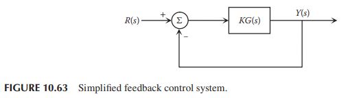
Consider the feedback control system in Figure 10.63, where
K G(s)=K \frac{100}{s(s+5)(s+20)},
and K is assumed to be 1 . Plot the Bode magnitude and phase curves using MATLAB. Give comments on the stability of the closed-loop system.
Learn more on how do we answer questions.
Note that the Bode plot is drawn based on the loop gain
L(s)=K \frac{100}{s(s+5)(s+20)}
The MATLAB command used to sketch the Bode plot is bode. Assuming K=1, the following is the MATLAB session:
>> num = [100];
>> den = conv(conv([1 0],[1 5]),[1 20]);
>> sysL = tf(num,den);
>> bode(sysL);
As observed in Figure 10.72, the phase curve crosses -180^{\circ} at frequency 10 \mathrm{rad} / \mathrm{s}, and the corresponding magnitude is approximately -28 \mathrm{~dB}. This implies that a gain of 28 \mathrm{~dB} can be added before the magnitude plot reaches 0 \mathrm{~dB} at that frequency. Thus, the \mathrm{GM} is 28 \mathrm{~dB}. The magnitude curve crosses 0 \mathrm{~dB} at frequency 1 \mathrm{rad} / \mathrm{s}, and the corresponding phase is -104^{\circ}. This implies that a phase of 76^{\circ} can be subtracted before the phase plot reaches -180^{\circ}. Thus, the PM is 76^{\circ}.
According to Equations 10.61 and 10.62,
\begin{aligned} &\begin{cases}\mathrm{GM}>0 \mathrm{~dB} & \text { stable } \\ \mathrm{GM}=0 \mathrm{~dB} & \text { marginally stable } \qquad (10.61)\\ \mathrm{GM}<0 \mathrm{~dB} & \text { unstable }\end{cases} \\ \\ &\begin{cases}\mathrm{PM}>0^{\circ} & \text { stable } \\ \mathrm{PM}=0^{\circ} & \text { marginally stable } \qquad (10.62) \\ \mathrm{PM}<0^{\circ} & \text { unstable }\end{cases} \end{aligned}
the closed-loop system with the proportional controller K=1 is stable.
More information on stability can be extracted from the GM. Specifically, the GM when K=1 gives the stability range of K for which the proportional feedback control system is stable. In our case, \mathrm{GM}=28 \mathrm{~dB} or 25 , and this indicates that the closed-loop system is stable for 0<K<25. We can also use the MATLAB command margin as follows:
>> [gm,pm,wcg,wcp] = margin(sysL)
which returns GM, PM, and the associated frequencies as defined in Figure 10.72. In our case, the GM returned by the command margin is 25 . Note that the stability range of K can be determined in this way only for systems that change from being stable to unstable as K increases.
