Question 10.10: A homogeneous thin rod of mass m and length l is connected t...
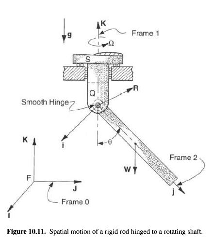
A homogeneous thin rod of mass m and length \mathcal{l} is connected to a vertical shaft S by a smooth hinge bearing at \mathcal{Q}. The shaft rotates with a constant angular velocity Ω, as shown in Fig. 10.11. (i) Derive the equation of motion of the rod. (ii) Determine as a function of θ the hinge bearing reaction torque exerted on the rod at \mathcal{Q}, for the initial data \dot{\theta}(0)=0 \text { at } \theta(0)=\theta_0 . (iii) Analyze the infinitesimal stability of the relative equilibrium states of the rod.
Learn more on how we answer questions.
(i). The central point \mathcal{Q} at the hinge being fixed in the inertial (machine) frame 0=\left\{F ; \mathbf{I} _k\right\}, the equation of motion for the rod is obtained from Euler’s law (10.66) in the principal body frame 2 = \left\{\mathcal{Q ; \mathbf{i}_{k}}\right\} . We need \mathbf{ω} , \mathbf{I}_{\mathcal{Q}},\text{ and } \mathbf{M}_{\mathcal{Q}}.
M_1^Q=I_{11}^Q \dot{\omega}_1+\omega_2 \omega_3\left(I_{33}^Q-I_{22}^Q\right),
M_2^Q=I_{22}^Q \dot{\omega}_2+\omega_3 \omega_1\left(I_{11}^Q-I_{33}^Q\right), (10.66)
M_3^Q=I_{33}^Q \dot{\omega}_3+\omega_1 \omega_2\left(I_{22}^Q-I_{11}^Q\right).
Let \mathbf{k} = \mathbf{i} _3 denote the hinge axis at \mathcal{Q}. Then the total angular velocity \omega ≡ \omega_{20} of the rod (frame 2) relative to the machine (frame 0) is the sum of the angular velocity \omega _{21}=\dot{\theta} \mathbf{k} of the rod relative to the vertical shaft (frame 1 ) and the angular velocity \omega _{10}= \Omega =\pmb{\Omega} \mathbf{K} of the shaft relative to the machine. Thus, referred to the rod frame 2,
\omega =-\Omega(\sin \theta \mathbf{i} +\cos \theta \mathbf{j} )+\dot{\theta} \mathbf{k}, (10.80a)
and hence the total angular acceleration of the rod is
\dot{\omega}=-\Omega \dot{\theta}(\cos \theta \mathbf{i} -\sin \theta \mathbf{j} )+\ddot{\theta} \mathbf{k}. (10.80b)
The rod frame at \mathcal{Q} is a principal body frame relative to which
\mathbf{I} _Q=\frac{1}{3} m \ell^2\left( \mathbf{i} _{11}+ \mathbf{i} _{33}\right) (10.80c)
in accordance with (9.46d), with a change of axes in mind. Finally, the moment of the forces and torques acting on the rod about Q is
\mathbf{I} _H\left( \mathcal{B} _r\right)=\frac{m \ell^2}{3}\left( \mathbf{i}_{11}+ \mathbf{i}_{22}\right) (9.46d)
\mathbf{M} _\mathcal{Q}=\mu_1 \mathbf{i} +\mu_2 \mathbf{j} – m g \frac{\ell}{2} \sin \theta \mathbf{k} . (10.80d)
Here \mu_1 \text { and } \mu_2 are unknown components of the torque exerted on the rod by the smooth hinge bearing for which \mu_3=0, and the weight W of the homogeneous rod acts at its center of mass at \mathbf{x} ^*=\ell / 2 \mathbf{j} .
Use of (10.80a) through (10.80d) in Euler’s equations (10.66) yields the components of the smooth hinge bearing reaction torque exerted on the rod at Q,
\mu_1=-\frac{2}{3} m \ell^2 \Omega \dot{\theta} \cos \theta, \quad \mu_2=\mu_3=0 (10.80e)
and the different ial equation of motion of the rod,
\ddot{\theta}+\left(p^2-\Omega^2 \cos \theta\right) \sin \theta=0, \quad p^2 \equiv \frac{3 g}{2 \ell} . (10.80f)
With the aid of this result, the reader may now determine from Euler’ s first law the resultant hinge reaction force R at Q.
When Ω = 0, \mu_{1} = 0 and ( 10.80f) reduces to the familiar pendulum equation.
In this case, the circular frequency p for the rod is the same as that of a simple pendulum of length L = 2l/3. Therefore, the exact and approximate solutions for the vibration of the rod when Ω = 0 may be read from those for the simple pendulum. We next consider the case when Ω ≠ 0.
(ii).
To determine the hinge bearing reaction torque (10.80e) as a function of θ, we need \dot{\theta}(\theta), the first integral of (10.80f). With \ddot{\theta}=d\left(\frac{1}{2} \dot{\theta}^2\right) / d \theta,
separation of the variables and use of the initial data \dot{\theta}(0) = 0 \text{ at } \theta(0) = \theta_{0} yields
\dot{\theta}= \pm \sqrt{\Omega^2\left(\cos ^2 \theta_0-\cos ^2 \theta\right)+3 \frac{g}{\ell}\left(\cos \theta-\cos \theta_0\right)} (10.80g)
Substitution of this result into (10.80e) delivers as a function of 0 the hinge bearing
reaction torque exerted on the rod at Q:
Notice that the reaction torque \mu_{1}(\theta) vanishes when \theta=\theta_0 or nπ/2 (n odd) and, of course, also when Ω =o.
(iii). The relative equilibrium states \theta_{s} of the rod, by (10.80f), are given by
\left(p^2-\Omega^2 \cos \theta_s\right) \sin \theta_s=0, (10.80i)
which yields three distinct states
\theta_s=0, \pi, \quad \theta_s=\cos ^{-1}\left(\frac{p^2}{\Omega^2}\right) . (10.80j)
To examine the infinitesimal stability of these states , introduce \theta = \theta_{s} + δ, where δ is an infinitesimal angular disturbance from \theta_{s} Then recalling (10.80i) and retaining only terms of the first order in δ, we obtain from (10.80f),
\ddot{\delta}+\left\{\left[p^2-\Omega^2 \cos \theta_s\right] \cos \theta_s+\Omega^2 \sin ^2 \theta_s\right\} \delta=0. (10.80k)
Therefore, the disturbance is bounded and simple harmonic, and hence infinitesimally stable, if and only if the coefficient
\omega^2 \equiv\left[p^2-\Omega^2 \cos \theta_s\right] \cos \theta_s+\Omega^2 \sin ^2 \theta_s>0 . (10.80l)
We now recall (10.80j). First consider \theta_{s} = 0 Then (10.80l) requires \omega^{2} = p^2-\Omega^2>0. Hence, the relative equilibrium state \theta_{s} = 0 is infinitesimally stable if and only if \Omega<p=\Omega_c , the critical angular speed of the vertical shaft:
\Omega_c \equiv p=\sqrt{\frac{3 g}{2 \ell}}, (10.80m)
which is independent of the mass of the rod. In this case, the small amplitude circular frequency of the rod oscillations about the vertical state \theta_s=0 is \omega_v \equiv \left(p^2-\Omega^2\right)^{1 / 2} \text {. }
Of course, the inverted vertical configuration of the rod \theta_{s} = \pi is impractic al in respect of the suggested design in Fig. 10.11. Even so, (10.80l) fails for \theta_{s} = \pi , and hence the inverted relative equilibrium state of the rod is inherently unstable for all angular speeds of the vertical shaft.
Notice that when \Omega=\Omega_c=p, \omega^2 \leq 0 for all positions (10.80j ). Hence, no infinitesimally stable relative equilibrium states of the rod exist at the critical angular speed \Omega=\Omega_c.
Finally, consider the case \cos \theta_s=p^2 / \Omega^2 This requires p/ Ω < l ; hence (10.80l) is satisfied, and the relative equilibrium state \theta_{s} = cos^{- 1}(p^2/ \Omega^2), regardless of the mass of the rod, is infinitesimally stable if and only if \Omega>p=\Omega_c. The small amplitude vibrational frequency of the rod about this displaced relative equilibrium state is \omega_d \equiv \Omega\left(1-p^4 / \Omega^4\right)^{1 / 2}.
In sum, if \Omega<\Omega_c, the vertical relative equilibrium position of the rod is its only infinitesimally stable relative equilibrium state. When the vertical shaft attains its critical angular speed, \Omega =\Omega_c , however, no infinitesimally stable relative equilibrium positions of the rod exist. Afterwards, when \Omega >\Omega_c, the displaced configuration of the rod at \theta_s=\cos ^{-1}\left(p^2 / \Omega^2\right) is its only infinitesimally stable relative equilibrium position.