Question 7.SP.3: Draw the shear and bending-moment diagrams for the beam AB. ......
Draw the shear and bending-moment diagrams for the beam AB. The distributed load of 40 lb/in. extends over 12 in. of the beam from A to C, and the 400-lb load is applied at E.
STRATEGY: Again, consider the entire beam as a free body to find the reactions. Then cut the beam within each region of continuous load. This will enable you to determine continuous functions for shear and bending moment, which you can then plot on a graph.

Distributed load: 40 lb/in. over 12 in. from A to C
Load at point E: 400 lb.
Learn more on how we answer questions.
Final Answer
MODELING and ANALYSIS:
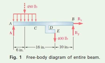
Free-Body, Entire Beam. Determine the reactions by considering the entire beam as a free body (Fig. 1).
+↺ \Sigma M_A=0: \quad B_y(32 ~\mathrm{in} .)-(480 ~\mathrm{lb})(6 ~\mathrm{in} .)-(400 ~\mathrm{lb})(22 ~\mathrm{in} .)=0
\begin{array}{ll} B_y=+365 ~\mathrm{lb} & \mathbf{B}_y=365 ~\mathrm{lb} \uparrow \end{array}
+↺ \Sigma M_B=0: \quad(480 ~\mathrm{lb})(26 ~\mathrm{in} .)+(400 ~\mathrm{lb})(10 ~\mathrm{in} .)-A(32 ~\mathrm{in} .)=0
A=+515 ~\mathrm{lb} \quad \mathbf{A}=515 ~\mathrm{lb} \uparrow
\stackrel{+}{\rightarrow} \Sigma F_x=0: \quad B_x=0 \quad \mathbf{B}_x=0
Now, replace the 400-lb load by an equivalent force-couple system acting on the beam at point D and cut the beam at several points (Fig. 2).
Shear and Bending Moment. From A to C. Determine the internal forces at a distance x from point A by considering the portion of the beam to the left of point 1. Replace that part of the distributed load acting on the free body by its resultant. You get
+\uparrow \Sigma F_y=0: \quad 515-40 x-V=0 \quad V=515-40 x
+↺ \Sigma M_1=0: \quad-515 x+40 x\left(\frac{1}{2} x\right)+M=0 \quad M=515 x-20 x^2
Note that V and M are not numerical values, but they are expressed as functions of x. The free-body diagram shown can be used for all values of x smaller than 12 in., so the expressions obtained for V and M are valid throughout the region 0 > x > 12 in.
From C to D. Consider the portion of the beam to the left of point 2. Again replacing the distributed load by its resultant, you have
+\uparrow \Sigma F_y=0: \quad 515-480-V=0 \quad V=35 ~\mathrm{lb}
+↺ \Sigma M_2=0:-515 x+480(x-6)+M=0 \quad M=(2880+35 x) ~\mathrm{lb} \cdot \text { in. }
These expressions are valid in the region 12 in. < x < 18 in.
From D to B. Use the portion of the beam to the left of point 3 for the region 18 in. < x < 32 in. Thus,
+\uparrow \Sigma F_y=0: \quad 515-480-400-V=0 \quad V=-365 ~\mathrm{lb}
+↺ \Sigma M_3=0: \quad-515 x+480(x-6)-1600+400(x-18)+M=0
M=(11,680-365 x) ~\mathrm{lb} \cdot \mathrm{in}.
Shear and Bending-Moment Diagrams. Plot the shear and bending- moment diagrams for the entire beam. Note that the couple of moment 1600 lb·in. applied at point D introduces a discontinuity into the bendingmoment diagram. Also note that the bending-moment diagram under the distributed load is not straight but is slightly curved.
REFLECT and THINK: Shear and bending-moment diagrams typically feature various kinds of curves and discontinuities. In such cases, it is often useful to express V and M as functions of location x as well as to determine certain numerical values.