Question 27.9: The flat panel shown in Fig. P.27.9 comprises a sheet of uni......
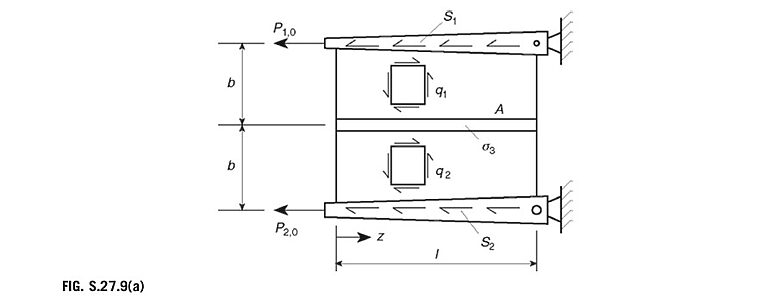
The flat panel shown in Fig. P.27.9 comprises a sheet of uniform thickness t, a central stringer of constant area A, and edge members of varying area. The panel is supported on pinned supports and is subjected to externally applied shear flows S_{1}\operatorname{and}S_{2}, together with end loads P_{1,0}\;\mathrm{and}\;P_{2,0}, as shown. The areas of the edge members vary such that the direct stresses \sigma_{1} and \sigma_{2} in the edge members are constant. Assuming that transverse strains are prevented, that the sheet transmits shear stress only, and that each part has suitable end members to take the complementary shear stresses, derive expressions for the variation of direct stress \sigma_{3} in the stringer and for the variation of shear flow in the upper panel in terms of the dimensions given and the elastic moduli E and G for the material.

Learn more on how do we answer questions.
The panel is unsymmetrical so that the shear flows in the top and bottom halves will have different values as shown in Fig. S.27.9(a).
For equilibrium of the element of the top member shown in Fig. 27.9(b),
i.e.,
{\frac{\partial P_{1}}{\partial z}}=S_{1}+q_{1} (i)
Similarly, for the equilibrium of the element of the central stringer shown in Fig. S.27.9(c),
P_{3}+{\frac{\partial P_{3}}{\partial z}}\delta z-P_{3}-q_{2}\delta z+q_{1}\delta z=0i.e.,
{\frac{\partial P_{3}}{\partial z}}=q_{2}-q_{1} (ii)
Also, from Fig. S.27.9(d),
P_{2}+{\frac{\partial P_{2}}{\partial z}}\delta z-P_{2}-S_{2}\delta z+q_{2}\delta z=0whence,
{\frac{\partial P_{2}}{\partial z}}=S_{2}-q_{2} (iii)
Now, from the longitudinal equilibrium of a length z of the panel (Fig. S.27.9(e)),
P_{1}+P_{3}+P_{2}-P_{1,0}-P_{2,0}-S_{1}z-S_{2}z=0i.e.,
P_{1}+P_{3}+P_{2}=P_{1,0}+P_{2,0}+(S_{1}+S_{2})z (iv)
and from its moment equilibrium about the bottom edge member,
P_{1}2b+P_{3}b-P_{1,0}2b-S_{1}z2b=0i.e.,
2P_{1}+P_{3}=2P_{1,0}+2S_{1}z (v)
From the compatibility condition between elements of the top edge member and the central stringer in Fig. S.27.9(f),
(1+\varepsilon_{1})\delta z=(1+\varepsilon_{3})\delta z+b\left({\frac{\mathrm{d}\gamma_{1}}{\mathrm{d}z}}+{\frac{\partial^{2}\nu}{\partial z^{2}}}\right)\delta zor
{\frac{\mathrm{d}\gamma_{1}}{\mathrm{d}z}}={\frac{1}{b}}(e_{1}-e_{3})-{\frac{\partial^{2}\nu}{\partial z^{2}}} (vi)
Similarly for elements of the central stringer and the bottom edge member,
{\frac{\mathrm{d}\gamma_{2}}{\mathrm{d}z}}={\frac{1}{b}}(\varepsilon_{3}-\varepsilon_{2})-{\frac{\partial^{2}\nu}{\partial z^{2}}} (vii)
Subtracting Eq. (vii) from (vi),
{\frac{\mathrm{d}\gamma_{1}}{\mathrm{d}z}}-{\frac{\mathrm{d}\gamma_{2}}{\mathrm{d}z}}={\frac{1}{b}}(\varepsilon_{1}-2\varepsilon_{3}+\varepsilon_{2}) (viii)
Now \gamma=q/G t,\,\varepsilon_{1}\!=\sigma_{1}/E,\,\varepsilon_{3}\!=\sigma_{3}/E,\,\mathrm{and~}\varepsilon_{2}\!=\sigma_{2}/E. Eq. (viii) may then be written as
{\frac{\mathrm{d}q_{1}}{\mathrm{d}z}}-{\frac{\mathrm{d}q_{2}}{\mathrm{d}z}}={\frac{G t}{b E}}(\sigma_{1}-2\sigma_{3}+\sigma_{2})or, from Eq. (i),
-{\frac{\partial^{2}P_{3}}{\partial z^{2}}}={\frac{G t}{b E}}(\sigma_{1}-2\sigma_{3}+\sigma_{2})Then, since \sigma_{3}=P_{3}/A,
{\frac{\partial^{2}\sigma_{3}}{\partial z^{2}}}={\frac{G t}{b E A}}(2\sigma_{3}-\sigma_{1}-\sigma_{2})or
{\frac{\partial^{2}\sigma_{3}}{\partial z^{2}}}-{\frac{2G t}{b E A}}\sigma_{3}={\frac{G t}{b E A}}(\sigma_{1}+\sigma_{2}) (ix)
The solution of Eq. (ix) is
\sigma_{3}=C\cosh\mu z+D\sinh\mu z+(\sigma_{1}+\sigma_{2})/2where \mu^{2}=2G t/b E A.
When z=0,\,\sigma_{3}=0\mathrm{~so~that~}C=-\,(\sigma_{1}+\sigma_{2})/2. When z=l,\,\sigma_{3}=0, which gives
D={\frac{(\sigma_{1}+\sigma_{2})}{2\sinh\mu l}}(\cosh\mu l-1)Thus,
\sigma_{3}=\left({\frac{\sigma_{1}+\sigma_{2}}{2}}\right)\left[1-\cosh\mu z-{\frac{(1-\cosh\mu l)}{\sinh\mu l}}\sinh\mu z\right] (x)
From Eq. (i),
q_{1}={\frac{\partial P_{1}}{\partial z}}-S_{1} (xi)
Substituting for {\mathbf{}}P_{1} from Eq. (v) in (xi),
q_{1}=-\frac{1}{2}\frac{\partial P3}{\partial z}=-\frac{1}{2}A\frac{\partial\sigma_{3}}{\partial z}Therefore, from Eq. (x),
q_{1}=A\left({\frac{\sigma_{1}+\sigma_{2}}{4}}\right)\mu\left[\sinh\mu z+{\frac{(1-\cosh\mu l)}{\sinh\mu l}}\cosh\mu z\right]