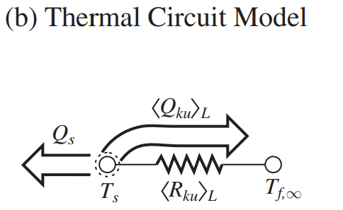
(a) The thermal circuit diagram is shown in Figure (b).
(b) The rate of surface-convection heat transfer is again given by A_{ku}=Lw, \left\langle Q_{ku}\right\rangle _{L}=\frac{T_{s}-T_{f,\infty }}{\left\langle R_{ku}\right\rangle_{L} } =A_{ku}\left\langle Nu\right\rangle _{L}\frac{k_{f}}{L} (T_{s}-T_{f,\infty }) as
\left\langle Q_{ku}\right\rangle _{L} =A_{ku}\left\langle q_{ku}\right\rangle_{L} =A_{ku}\left\langle Nu\right\rangle _{L}\frac{k_{f}}{L} (T_{s}-T_{f,\infty })
Where
A_{ku} = L^{2}
For an isothermal, semi-infinite plate, we have the relation for \left\langle Nu\right\rangle _{L} given by
\left\langle Nu\right\rangle _{L}=(\left\langle Nu_{L,l}\right\rangle ^{6}+\left\langle Nu_{L,t}\right\rangle ^{6})^{1/6},
\left\langle Nu_{L,l}\right\rangle=\frac{2.8}{ln[1+2.8/(a_{1}Ra_{L}^{1/4})]} ,
\left\langle Nu_{L,t}\right\rangle=\frac{0.13Pr^{0.22}}{(1+0.61Pr^{0.81})^{0.42}} Ra_{L}^{1/3} ,
a_{1}=\frac{4}{3}\frac{0.503}{[1+(0.492/Pr)^{9/16}]^{4/9}}
and the Rayleigh number Ra_{L}, from Ra_{L}\equiv Gr_{L}Pr=\frac{g\beta _{f}(T_{s}-T_{f,\infty })L^{3}}{v_{f}\alpha _{f}} is
Ra_{L}=\frac{g\beta _{f}(T_{s}-T_{f,\infty })L^{3}}{v_{f}\alpha _{f}}
Using Table for water (at T = 330 K), and g = 9.807 m/s^{2}, we have
\beta _{f} = 0.000273 1/K Table (at T = 310 K, the closest data available)
k_{f} = 0.648 W/m-K Table
\alpha _{f} = 1.54 × 10^{−7} m^{2}/s Table
ν_{f} = 5.05 × 10^{−7} m^{2}/s Table
Pr = 3.22 Table .
Then
Ra_{L}=\frac{9.807(m/s^{2}) × 0.000273(1/K) × (95 − 20)(K) × (0.2)^{3} (m^{3} )}{5.05 × 10^{−7} (m^{2}/s) × 1.54 × 10^{−7} (m^{2}/s)}
= 2.066 × 10^{10} turbulent, thermobuoyant flow.
The \left\langle Nu\right\rangle _{L} relation \left\langle Nu\right\rangle _{L}=(\left\langle Nu_{L,l}\right\rangle ^{6}+\left\langle Nu_{L,t}\right\rangle ^{6})^{1/6} ,\left\langle Nu_{L,l}\right\rangle=\frac{2.8}{ln[1+2.8/(a_{1}Ra_{L}^{1/4})]} ,\left\langle Nu_{L,t}\right\rangle=\frac{0.13Pr^{0.22}}{(1+0.61Pr^{0.81})^{0.42}} Ra_{L}^{1/3} ,a_{1}=\frac{4}{3}\frac{0.503}{[1+(0.492/Pr)^{9/16}]^{4/9}} is
\left\langle Nu\right\rangle _{L}=[( Nu_{L,l}) ^{6}+( Nu_{L,t}) ^{6}]^{1/6}
\left\langle Nu_{L,l}\right\rangle=\frac{2.8}{ln(1+2.8/a_{1}Ra^{1/4})}
\left\langle Nu_{L,t}\right\rangle=\frac{0.13Pr^{0.22}}{(1+0.61Pr^{0.81})^{0.42}} Ra_{L}^{1/3}
a_{1}=\frac{4}{3}\frac{0.503}{[1+(0.492/Pr)^{9/16}]^{4/9}}
Then
a_{1} = 0.5874
\left\langle Nu_{L,l}\right\rangle=\frac{2.8}{ln [ 1 + 2.8/0.5874(2.066 × 10^{10})^{1/4}]}
= 224.1
\left\langle Nu_{L,t}\right\rangle=\frac{0.13×(3.22)^{0.22}}{[1 + 0.61(3.22)^{0.81}]^{ 0.42} } (2.066 × 10^{10})^{ 1/3}
= \frac{0.1681 }{1.487} × 2.744 × 10^{3} = 310.0
\left\langle Nu\right\rangle _{L}=[( 224.1) ^{6}+( 310.0) ^{6}]^{1/6}
= 317.0
The surface-convection heat transfer rate is
\left\langle Q_{ku}\right\rangle _{L}= (0.2)^{2} (m^{2} ) × 317.0 × \frac{0.648(W/m-K) }{0.2(m)} × (95 − 20)(K)
= 3, 081 W
(c) The average surface-convection resistance \left\langle R_{ku}\right\rangle _{L} is given by A_{ku}=Lw, \left\langle Q_{ku}\right\rangle _{L}=\frac{T_{s}-T_{f,\infty }}{\left\langle R_{ku}\right\rangle_{L} } =A_{ku}\left\langle Nu\right\rangle _{L}\frac{k_{f}}{L} (T_{s}-T_{f,\infty }), i.e.,
\left\langle R_{ku}\right\rangle _{L}=\frac{T_{s}-T_{f,\infty }}{\left\langle Q_{ku}\right\rangle_{L} }=\frac{(95 − 20)(^{\circ }C)}{3.081 × 10^{3} (W)} = 0.02434^{\circ }C/W
A_{ku}\left\langle R_{ku}\right\rangle _{L} = (0.2)^{2} (m^{2}) × 0.02434(^{\circ }C/W) = 9.737 × 10^{−4\circ } C/(W/m^{2}).
(d) Comparing thermobuoyant, forced-parallel, and forced-perpendicular flows, the thermobuoyant flow is the least effective (\left\langle R_{ku}\right\rangle _{L} = 0.02434^{\circ}C/W), followed by laminar and turbulent forced parallel (\left\langle R_{ku}\right\rangle _{L} = 0.001769^{\circ}C/W and \left\langle R_{ku}\right\rangle _{L} = 0.001654^{\circ}C/W), with the single-jet perpendicular flow being the most effective (\left\langle R_{ku}\right\rangle _{L}= 0.00003976^{\circ}C/W) among them.