Question 9.8: Use a Δ-to-Y impedance transformation to find I0,I1,I2,I3,I4...

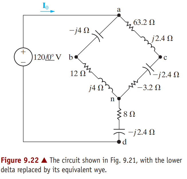
First note that the circuit is not amenable to series or parallel simplification as it now stands. A Δ -to-Y impedance transformation allows us to solve for all the branch currents without resorting to either the node-voltage or the mesh-current method. If we replace either the upper delta (abc) or the lower  delta (bcd) with its Y equivalent, we can further simplify the resulting circuit by series-parallel combinations. In deciding which delta to replace, the sum of the impedances around each delta is worth checking because this quantity forms the denominator for the equivalent Y impedances. The sum around the lower delta is so we choose to eliminate it from the circuit. The Y impedance connecting to terminal b is

Z_{1} =\frac{(20 + j60)(10)}{30 + j40} = 12 + j4Ω,

the Y impedance connecting to terminal c is

Z_{2} =\frac{10( – j20)(10)}{30 + j40} = -3.2 – j 2.4 Ω,

and the Y impedance connecting to terminal d is

Z_{3} =\frac{(20 + j60)( – j20)}{30 + j40} =8 – j 24 Ω,

Inserting the Y-equivalent impedances into the circuit, we get the circuit shown in Fig 9.22, which we can now simplify by series-parallel reductions. The impedence of the abn branch is

Z_{abn} = 12+ j4- j4=12Ω,

and the impedance of the acn branch is

Z_{acn} =  63.2 + j 2.4 – j 2.4 – 3.2 = 60Ω.

Note that the abn branch is in parallel with the acn branch. Therefore we may replace these two branches with a single branch having an impedance of

Z_{an} =\frac{(60)( 12)}{72} =10 Ω,

Combining this 10 Ω resistor with the impedance between n and d reduces the circuit shown in Fig. 9.22 to the one shown in Fig. 9.23. From the latter circuit,

\pmb{I}_{0} =\frac{120 \angle 0^{°}}{18 – j 24} = 4 \angle 53.13^{°}= 2.4 + j 3.2 A.

Once we know\pmb{I}_{0} we can work back through the equivalent circuits to find the branch currents in the original circuit. We begin by noting that \pmb{I}_{0}   is the current in the branch nd of Fig. 9.22. Therefore

\pmb{V}_{nd} = (8 – j 24)\pmb{I}_{0} = 96 – j 32 V.

We may now calculate the voltage \pmb{V}_{an}  because

\pmb{V}=\pmb{V}_{an}+\pmb{V}_{nd} .

and both V and \pmb{V}_{nd} are known. Thus

\pmb{V}_{an}= 120 – 96 + j 32 = 24 + j 32 V.

We now compute the branch currents \pmb{I}_{abn} and \pmb{I}_{acn} :

\pmb{I}_{abn} =\frac{24+j32}{12} =2 + j\frac{8}{3}A,

\pmb{I}_{acn} =\frac{24+j32}{60} =\frac{4}{10} + j\frac{8}{15}A.

In terms of the branch currents defined in Fig. 9.21,

\pmb{I}_{1} =\pmb{I}_{abn}=2 + j\frac{8}{3}A,

\pmb{I}_{2} =\pmb{I}_{acn} =\frac{4}{10} + j\frac{8}{15}A.

We check the calculations of \pmb{I}_{1} and   \pmb{I}_{2} by noting that

\pmb{I}_{1} + \pmb{I}_{2} = 2.4 + j 3.2 = \pmb{I}_{0}.

To find the branch currents \pmb{I}_{3},\pmb{I}_{4},and \pmb{I}_{5}  we must first calculate the voltages \pmb{V}_{1}and \pmb{V}_{2} Refering to Fig. 9.21, we note that

\pmb{V}_{1} =120 \angle 0^{°}- (-j4) \pmb{I}_{1}=\frac{328}{3} + j8 V, .

\pmb{V}_{2} =120 \angle 0^{°}- (63.2 + j 2.4) \pmb{I}_{2}= 96 – j\frac{104}{3}  V.

We now calculate the branch currents \pmb{I}_{3},\pmb{I}_{4},and \pmb{I}_{5}  :

\pmb{I}_{3}=\frac{V_{1}-V_{2}}{10}=\frac{4}{3}+ j\frac{12.8}{3}A,

\pmb{I}_{4}=\frac{V_{1}}{20+j60}=\frac{2}{3}- j1.6A,

\pmb{I}_{4}=\frac{V_{2}}{-j20}=\frac{26}{15}+ j4.8 A.

We check the calculations by noting that

\pmb{I}_{3}+ \pmb{I}_{2}=\frac{4}{3}+\frac{4}{10} + j\frac{12.8}{3} + j\frac{8}{15}=\frac{26}{15}+ j4.8 = \pmb{I}_{5} .