Equation 4–44 is to be proven.
\frac{d B_{ sys }}{d t}=\frac{d}{d t} \int_{ CV } \rho b d V+\int_{ CS } \rho b \vec{V}_{r} \cdot \vec{n} d A (4-44)
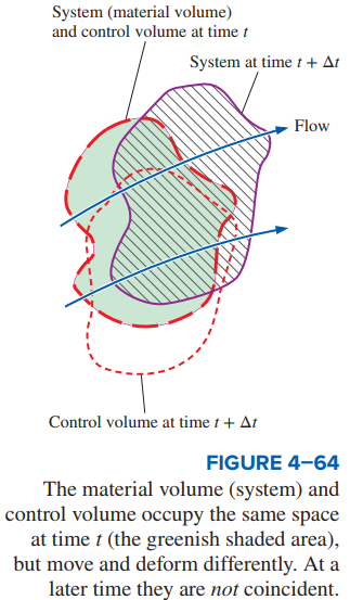
Analysis The general three-dimensional version of the Leibniz theorem, Eq. 4–50, applies to any volume. We choose to apply it to the control volume of interest, which can be moving and/or deforming differently than the material volume (Fig. 4–64). Setting G to 𝜌b, Eq. 4–50 becomes
\frac{d}{d t} \int_{V(t)} G(x, y, z, t) d V=\int_{V(t)} \frac{\partial G}{\partial t} d V+\int_{A(t)} G \vec{V}_{A} \cdot \vec{n} d A (4-50)
\frac{d}{d t} \int_{ CV } \rho b d V =\int_{ CV } \frac{\partial}{\partial t}(\rho b) d V +\int_{ CS } \rho b \vec{V}_{ CS } \cdot \vec{n} d A (1)
We solve Eq. 4–53 for the control volume integral,
\frac{d B_{ sys }}{d t}=\int_{ CV } \frac{\partial}{\partial t}(\rho b) d V+\int_{ CS } \rho b \vec{V} \cdot \vec{n} d A (4-53)
\int_{ CV } \frac{\partial}{\partial t}(\rho b) d V =\frac{d B_{ sys }}{d t}-\int_{ CS } \rho b \vec{V} \cdot \vec{n} d A (2)
Substituting Eq. 2 into Eq. 1, we get
\frac{d}{d t} \int_{ CV } \rho b d V=\frac{d B_{ sys }}{d t}-\int_{ CS } \rho b \vec{V} \cdot \vec{n} d A+\int_{ CS } \rho b \vec{V}_{ CS } \cdot \vec{n} d A (3)
Combining the last two terms and rearranging,
\frac{d B_{ sys }}{d t}=\frac{d}{d t} \int_{ CV } \rho b d V+\int_{ CS } \rho b\left(\vec{V}-\vec{V}_{ CS }\right) \cdot \vec{n} d A (4)
But recall that the relative velocity is defined by Eq. 4–43. Thus,
\vec{V}_{r}=\vec{V}-\vec{V}_{ CS } (4-43)
RTT in terms of relative velocity:
\frac{d B_{ sys }}{d t}=\frac{d}{d t} \int_{ CV } \rho b d V+\int_{ CS } \rho b \vec{V} \cdot \vec{n} d A (5)
Discussion Equation 5 is indeed identical to Eq. 4–44, and the power and elegance of the Leibniz theorem are demonstrated.
\frac{d B_{ sys }}{d t}=\frac{d}{d t} \int_{ CV } \rho b d V+\int_{ CS } \rho b \vec{V}_{r} \cdot \vec{n} d A (4-44)