SOLUTION We are to plot the mean boundary layer profile u( y) at the end of a flat plate using three different approximations.
Assumptions 1 The plate is smooth, but there are free-stream fluctuations that tend to cause the boundary layer to transition to turbulence sooner than usual—the boundary layer is turbulent from the beginning of the plate. 2 The flow is steady in the mean. 3 The plate is infinitesimally thin and is aligned parallel to the free stream.
Properties The kinematic viscosity of air at 20°C is \nu=1.516 \times 10^{-5} m ^{2} / s.
Analysis First we calculate the Reynolds number at x = L,
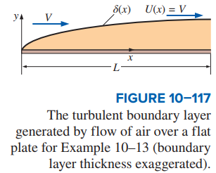
\operatorname{Re}_{x}=\frac{V x}{v}=\frac{(10.0 m / s )(15.2 m )}{1.516 \times 10^{-5} m ^{2} / s }=1.00 \times 10^{7}
This value of \operatorname{Re}_{x} is well above the transitional Reynolds number for a flat plate boundary layer (Fig. 10–81), so the assumption of turbulent flow from the beginning of the plate is reasonable.
Using the column (a) values of Table 10–4, we estimate the boundary layer thickness and the local skin friction coefficient at the end of the plate,
| TABLE 10–4 |
| Summary of expressions for laminar and turbulent boundary layers on a smooth flat plate aligned parallel to a uniform stream* |
| Property |
Laminar |
(a) Turbulent(†) |
(b) Turbulent(‡) |
| Boundary layer thickness |
\frac{\delta}{x}=\frac{4.91}{\sqrt{\operatorname{Re}_{x}}} |
\frac{\delta}{x}\cong\frac{0.16}{\left(\operatorname{Re}_{x}\right)^{1/7}} |
\frac{\delta}{x}\cong\frac{0.38}{\left(\operatorname{Re}_{x}\right)^{1/5}} |
| Displacement thickness |
\frac{\delta*}{x}=\frac{1.72}{\sqrt{\operatorname{Re}_{x}}} |
\frac{\delta^{*}}{x}\cong\frac{0.020}{\left(\operatorname{Re}_{x}\right)^{1/7}} |
\frac{\delta^{*}}{x}\cong\frac{0.048}{\left(\operatorname{Re}_{x}\right)^{1/5}} |
| Momentum thickness |
\frac{\theta}{x}=\frac{0.664}{\sqrt{\operatorname{Re}_{x}}} |
\frac{\theta}{x}\cong\frac{0.016}{\left(\operatorname{Re}_{x}\right)^{1/7}} |
\frac{\theta}{x}\cong\frac{0.037}{\left(\operatorname{Re}_{x}\right)^{1/5}} |
| Local skin friction coefficient |
C_{f, x}=\frac{0.664}{\sqrt{\operatorname{Re}_{x}}} |
C_{f,x}\cong\frac{0.027}{\left(\operatorname{Re}_{x}\right)^{1/7}} |
C_{f, x} \cong \frac{0.059}{\left( Re _{x}\right)^{1 /5}} |
| * Laminar values are exact and are listed to three significant digits, but turbulent values are listed to only two significant digits due to the large uncertainty affiliated with all turbulent flow fields. |
| † Obtained from one-seventh-power law. |
| ‡ Obtained from one-seventh-power law combined with empirical data for turbulent flow through smooth pipes. |
\delta \cong \frac{0.16 x}{\left(\operatorname{Re}_{x}\right)^{1 / 7}}=0.240 m \quad C_{f, x} \cong \frac{0.027}{\left(\operatorname{Re}_{x}\right)^{1 / 7}}=2.70 \times 10^{-3} (1)
We calculate the friction velocity by using its definition (Eq. 10–84) and the definition of C_{f, x} (left part of Eq. 10 of Example 10–10),
Friction velocity: u_{*}=\sqrt{\frac{\tau_{w}}{\rho}} (E. 10-84)
u_{*}=\sqrt{\frac{\tau_{w}}{\rho}}=U \sqrt{\frac{C_{f, x}}{2}}=(10.0 m / s ) \sqrt{\frac{2.70 \times 10^{-3}}{2}}=0.367 m / s (2)
where U = constant = V everywhere for a flat plate. It is trivial to generate a plot of the one-seventh-power law (Eq. 10–82), but the log law (Eq. 10–83) is implicit for u as a function of y. Instead, we solve Eq. 10–83 for y as a function of u,
\frac{u}{U} \cong\left(\frac{y}{\delta}\right)^{1 / 7} \quad \text { for } y \leq \delta, \quad \rightarrow \quad \frac{u}{U} \cong 1 \quad \text { for } y>\delta (Eq. 10-82)
The log law: \frac{u}{u_{*}}=\frac{1}{\kappa} \ln \frac{y u_{*}}{v}+B (Eq. 10-83)
y=\frac{v}{u_{*}} e^{\kappa\left(u / u_{*}-B\right)} (3)
Since we know that u varies from 0 at the wall to U at the boundary layer edge, we are able to plot the log law velocity profile in physical variables using Eq. 3. Finally, Spalding’s law of the wall (Eq. 10–85) is also written in terms of y as a function of u. We plot all three profiles on the same plot for comparison (Fig. 10–118). All three are close, and we cannot distinguish the log law from Spalding’s law on this scale.
\frac{y u_{*}}{v}=\frac{u}{u_{*}}+e^{-\kappa B}\left[e^{\kappa\left(u / u_{*}\right)}-1-\kappa\left(u / u_{*}\right)-\frac{\left[\kappa\left(u / u_{*}\right)\right]^{2}}{2}-\frac{\left.\left[\kappa\left(u / u_{*}\right)\right]^{3}\right]}{6}\right] (Eq. 10-85)
Instead of a physical variable plot with linear axes as in Fig. 10–118, a semi-log plot of nondimensional variables is often drawn to magnify the near-wall region. The most common notation in the boundary layer literature for the nondimensional variables is y^{+} \text {and } u^{+} (inner variables or law of the wall variables), where
Law of the wall variables: y^{+}=\frac{y u_{*}}{v} \quad u^{+}=\frac{u}{u_{*}} (4)
As you can see, y^{+} is a type of Reynolds number, and friction velocity u* is used to nondimensionalize both y and u. Figure 10–118 is redrawn in Fig. 10–119 using law of the wall variables. The differences between the three approximations, especially near the wall, are much clearer when plotted in this fashion. Typical experimental data are also plotted in Fig. 10–119 for comparison. Spalding’s formula does the best job overall and is the only expression that follows experimental data near the wall. In the outer part of the boundary layer, the experimental values of u^{+} level off beyond some value of y^{+}, as does the one-seventh-power law. However, both the log law and Spalding’s formula continue indefinitely as a straight line on this semi-log plot.
Discussion Also plotted in Fig. 10–119 is the linear equation u^{+}=y^{+}. The region very close to the wall \left(0<y^{+}<5 \text { or } 6\right) is called the viscous sublayer. In this region, turbulent fluctuations are suppressed due to the close proximity of the wall, and the velocity profile is nearly linear. Other names for this region are linear sublayer and laminar sublayer. We see that Spalding’s equation captures the viscous sublayer and blends smoothly into the log law by about y^{+}=100. Neither the one-seventh-power law nor the log law is valid as we approach the wall.