Question 24.11: Repeat Example 24.10 for f = 10 kHz.
Repeat Example 24.10 for f = 10 kHz.
Learn more on how we answer questions.
T=\frac{1}{f}=\frac{1}{10 kHz }=0.1 ms.
and \frac{T}{2}=0.05 ms.
with \tau=t_{p}=\frac{T}{2}=0.05 ms.
In other words, the pulse width is exactly equal to the time constant of the network. The voltage v_{C} will not reach the final value before the first pulse of the square-wave input returns to zero volts.
\text { For } t \text { in the range } t=0 \text { to } T / 2, V_{i}=0 V \text { and } V_{f}=10 mV \text {, and }v_{C}=10 mV \left(1-e^{-t / \tau}\right).
\text { Recall from Chapter } 10 \text { that at } t=\tau, v_{C}=63.2 \% \text { of the final value. } Substituting t = τ into the equation above yields
v_{C}=(10 mV )\left(1-e^{-1}\right)=(10 mV )(1-0.368).
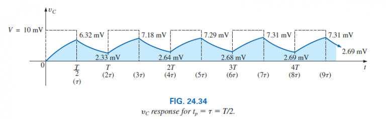
=(10 mV )(0.632)=6.32 mV.
as shown in Fig. 24.34.
\text { For the discharge phase between } t=T / 2 \text { and } T, V_{i}=6.32 mV \text { and }V_{f}=0 V , \text { and }
v_{C}=V_{f}+\left(V_{i}-V_{f}\right) e^{-t / \tau}.
=0 V +(6.32 mV -0 V ) e^{-t / \tau}.
v_{C}=6.32 mV e^{-t / \tau}.
with t now being measured from t = T/2 in Fig. 24.34. In other words, for each interval in Fig. 24.34, the beginning of the transient waveform is defined as t = 0 s. The value of v_{C} at t = T is therefore determined by substituting t=\tau \text { into the above equation, and not } 2 \tau as defined by Fig. 24.34.
\text { Substituting } t=\tau \text {, }v_{C}=(6.32 mV )\left(e^{-1}\right)=(6.32 mV )(0.368).
= 2.33 mV.
as shown in Fig. 24.34.
\text { For the next interval, } V_{i}=2.33 mV \text { and } V_{f}=10 mV \text {, and }v_{C}=V_{f}+\left(V_{i}-V_{f}\right) e^{-t / \tau}.
=10 mV +(2.33 mV -10 mV ) e^{-t / \tau}.
v_{C}=10 mV -7.67 mVe ^{-t / \tau}.
\text { At } t=\tau \text { (since } t=T=2 \tau \text { is now } t=0 s \text { for this interval), }.
v_{C}=10 mV -7.67 mV e^{-1}.
=10 mV -2.82 mV.
v_{C}=7.18 mV.
as shown in Fig. 24.34.
\text { For the discharge interval, } V_{i}=7.18 mV \text { and } V_{f}=0 V \text {, and }v_{C}=V_{f}+\left(V_{i}-V_{f}\right) e^{-t / \tau}.
=0 V +(7.18 mV -0) e^{-t / \tau}.
v_{C}=7.18 mV e^{-t / \tau}.
\text { At } t=\tau \text { (measured from } 3 \tau \text { in Fig. 24.34), }v_{C}=(7.18 mV )\left(e^{-1}\right)=(7.18 mV )(0.368).
= 2.64 mV.
as shown in Fig. 24.34.
Continuing in the same manner, the remaining waveform for v_{C} is generated as depicted in Fig. 24.34. Note that repetition occurs after t = 8τ, and the waveform has essentially reached steady-state conditions in a period of time less than 10τ, or five cycles of the applied square wave.
A closer look reveals that both the peak and the lower levels continued to increase until steady-state conditions were established. Since the exponential waveforms between t = 4T and t = 5T have the same time constant, the average value of v_{C} can be determined from the steady-state 7.31 mV and 2.69 mV levels as follows:
V_{ av }=\frac{7.31 mV +2.69 mV }{2}=\frac{10 mV }{2}=5 mV.
which equals the average value of the applied signal as stated earlier in
this section.
We can use the results in Fig. 24.34 to plot i_{C}. At any instant of time,
v_{i}=v_{R}+v_{C} \quad \text { or } \quad v_{R}=v_{i}-v_{C}.
and i_{R}=i_{C}=\frac{v_{i}-v_{C}}{R}.
\text { At } t=0^{+}, v_{C}=0 V , \text { and }.
i_{R}=\frac{v_{i}-v_{C}}{R}=\frac{10 mV -0}{5 k \Omega}=2 \mu A.
as shown in Fig. 24.35.
As the charging process proceeds, the current i_{C} decays at a rate determined by
i_{C}=2 \mu A e^{-t / \tau}.
\text { At } t=\tau.
i_{C}=(2 \mu A )\left(e^{-\tau / \tau}\right)=(2 \mu A )\left(e^{-1}\right)=(2 \mu A )(0.368).
=0.736 \mu A.
as shown in Fig. 24.35.
For the trailing edge of the first pulse, the voltage across the capacitor cannot change instantaneously, resulting in the following when v_{i} drops to zero volts:
i_{C}=i_{R}=\frac{v_{i}-v_{C}}{R}=\frac{0-6.32 mV }{5 k \Omega}=-1.264 \mu A.
as illustrated in Fig. 24.35. The current then decays as determined by
i_{C}=-1.264 \mu A e^{-t / \tau}.
\text { and at } t=\tau \text { (actually } t=2 \tau \text { in Fig. 24.35), }i_{C}=(-1.264 \mu A )\left(e^{-\tau / \tau}\right)=(-1.264 \mu A )\left(e^{-1}\right).
=(-1.264 \mu A )(0.368)=-0.465 \mu A.
as shown in Fig. 24.35.
\text { At } t=T(t=2 \tau), v_{C}=2.33 mV , \text { and } v_{i} \text { returns to } 10 mV , \text { resulting in }i_{C}=i_{R}=\frac{v_{i}-v_{C}}{R}=\frac{10 mV -2.33 mV }{5 k \Omega}=1.534 \mu A.
The equation for the decaying current is now
i_{C}=1.534 \mu A e^{-t / \tau}.
\text { and at } t=\tau \text { (actually } t=3 \tau \text { in Fig. 24.35), }.
i_{C}=(1.534 \mu A )(0.368)=0.565 \mu A.
The process continues until steady-state conditions are reached at the same time they were attained for v_{C}. Note in Fig. 24.35 that the positive peak current decreased toward steady-state conditions while the negative peak became more negative. Note that the current waveform becomes symmetrical about the axis when steady-state conditions are established.
The result is that the net average current over one cycle is zero, as it should be in a series R-C circuit. Recall from Chapter 10 that the capacitor under dc steady-state conditions can be replaced by an open-circuit equivalent, resulting in I_{C}=0 A.