Question 18.1: Determine the reactions and the force in each member of the ...

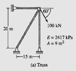
Degrees of Freedom From the analytical model of the truss shown in Fig. 18.11(b), we observe that only joint 3 is free to translate. Thus the truss has two degrees of freedom, d_1 and d_2, which are the unknown translations of joint 3 in the X and Y directions, respectively.

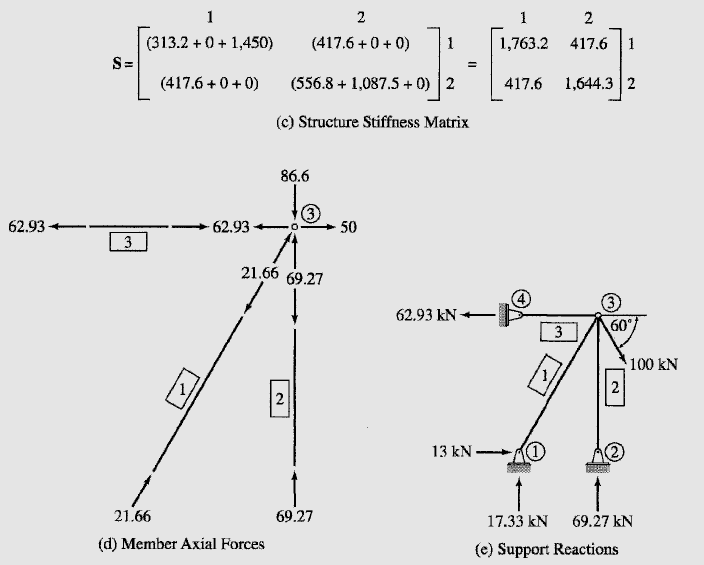
Structure Stiffness Matrix

Member 1 As shown in Fig. 18.11(b), joint 1 has been selected as the beginning joint and joint 3 as the end joint for member 1. By applying Eqs. (18.13), we determine

\cos θ = \frac{X_e – X_b}{L} = \frac{X_e – X_b}{\sqrt{(X_e – X_b)^2 + (Y_e – Y_b)^2}}                            (18.13a)

\sin θ = \frac{Y_e – Y_b}{L} = \frac{Y_e – Y_b}{\sqrt{(X_e – X_b)^2 + (Y_e – Y_b)^2}}                            (18.13b)

The member stiffness matrix in global coordinates can now be evaluated by using Eq. (18.29)

K = \frac{EA}{L}\begin{bmatrix} \cos^2 θ & \cos θ \sin θ& -\cos^2 θ & -\cos θ \sin θ\\ \cos θ \sin θ & \sin^2 θ & -\cos θ \sin θ & -\sin^2 θ\\-\cos^2 θ & -\cos θ \sin θ & \cos^2 θ & \cos θ \sin θ \\ -\cos θ \sin θ & -\sin^2 θ & \cos θ \sin θ & \sin^2 θ \end{bmatrix}           (18.29)

or

                       (1)

From Fig. 18.11(b), we observe that the displacements of the beginning joint 1 for the member are zero, whereas the displacements of the end joint 3 are d_1 and d_2. Thus the structure degree of freedom numbers for this member are 0, 0, 1, 2. These numbers are written on the right side and at the top of K_1 (see Eq. (1)) to indicate the rows and columns, respectively, of the structure stiffness matrix S, where the elements of K_1 must be stored. Note that the elements of K_1, which correspond to the zero structure degree of freedom number, are simply disregarded. Thus, the element in row 3 and column 3 of K_1 is stored in row 1 and column 1 of S, as shown in Fig. 18.11(c). Similarly, the element in row 3 and column 4 of K_1 is stored in row 1 and column 2 of S. The remaining elements of K_1 are stored in S in a similar manner (Fig. 18.11(c)).

Member 2 From Fig. 18.11(b), we can see that joint 2 is the beginning joint and joint 3 is the end joint for member 2. By applying Eqs. (18.13), we obtain

Thus, by using Eq. (18.29)

From Fig. 18.11(b), we can see that the structure degree of freedom numbers for this member are 0, 0, 1, 2. These numbers are used to store the pertinent elements of K_2 in their proper positions in the structure stiffness matrix S, as shown in Fig. 18.11(c).

Member 3       \cos θ = 1        \sin θ = 0

By using Eq. (18.29),

The structure degree of freedom numbers for this member are 0, 0, 1, 2. By using these numbers, the elements of K_3 are stored in S, as shown in Fig. 18.11(c).

Note that the structure stiffness matrix S (Fig. 18.11(c)), obtained by assembling the stiffness coefficients of the three members, is symmetric.

Joint Load Vector By comparing Fig. 18.11(a) and (b), we realize that

P_1 = 100 \cos 60° = 50 kN            P_2 = -100 \sin 60° = -86.6 kN

Thus the joint load vector is

P = \begin{bmatrix} 50 \\ -86.6 \end{bmatrix}                 (2)

Joint Displacements The stiffness relations for the entire truss can be expressed as (Eq. (18.41) with P_f = 0)

P – P_f = Sd                    (18.41)

P = Sd                              (3)

By substituting P from Eq. (2) and S from Fig. 18.11(c), we write Eq. (3) in expanded form as

By solving these equations simultaneously, we determine the joint displacements to be

d_1 = 0.0434 m                d_2 = -0.0637 m

or

Member End Displacements and End Forces

Member 1 The member end displacements in global coordinates, v, can be obtained by simply comparing the member’s global degree of freedom numbers with the structure degree of freedom numbers for the member, as follows:

v_1 = \begin{bmatrix} v_1 \\ v_2 \\ v_3\\ v_4\end{bmatrix} \begin{matrix}0 \\ 0 \\ 1 \\ 2\end{matrix} =\begin{bmatrix} 0 \\ 0 \\ d_1\\ d_2\end{bmatrix} = \begin{bmatrix}0\\ 0 \\ 0.0434 \\ -0.0637 \end{bmatrix} m                               (4)

Note that the structure degree of freedom numbers for the member (0, 0, 1, 2) are written on the right side of v, as shown in Eq. (4). Since the structure degree of freedom numbers corresponding to v1 and v2 are zero, this indicates that v_1 = v_2 = 0. Similarly, the numbers 1 and 2 corresponding to v_3 and v_4, respectively, indicate that v_3 = d_1 and v_4 = d_2. It should be realized that these compatibility equations could have been established alternatively simply by a visual inspection of the line diagram of the structure (Fig. 18.11(b)). However, the use of the structure degree of freedom numbers enables us conveniently to program this procedure on a computer.

The member end displacements in local coordinates can now be determined by using the relationship u = Tv (Eq. (18.14)), with T as defined in Eq. (18.22):

u = Tv                   (18.14)

T = \begin{bmatrix} \cos θ & \sin θ & 0 & 0 \\ 0& 0 & \cos θ & \sin θ \end{bmatrix}                         (18.22)

By using Eq. (18.7), we compute member end forces in local coordinates as

Q = ku                            (18.7)

Thus, as shown in Fig. 18.11(d), the axial force in member 1 is

21.66 kN (C)

By applying Eq. (18.17), we can determine member end forces in global coordinates as

F = T^T Q                        (18.17)

Member 2 The member end displacements in global coordinates are given by

By using the relationship u = Tv, we determine the member end displacements in local coordinates to be

Next, the member end forces in local coordinates are computed by using the relationship Q = ku:

Thus, as shown in Fig. 18.11(d), the axial force in member 2 is

69.27 kN (C)

By using the relationship F = T^T Q, we calculate the member end forces in global coordinates to be

Member 3

u = Tv

Q = ku

Thus, the axial force in member 3 is (Fig. 18.11(d))

62.93 kN (T)

Support Reactions As shown in Fig. 18.11(e), the reactions at the support joints 1, 2, and 4 are equal to the forces in global coordinates at the ends of the members connected to these joints.

Equilibrium Check Applying the equations of equilibrium to the free body of the entire structure (Fig. 18.11(e)), we obtain

+→∑F_X =0          13 – 62.93 + 100 \cos 60° = 0.07 ≈ 0                 Checks

+↑∑F_Y =0          17.33 + 69.27 – 100 \sin 60° = 0                         Checks

+\circlearrowleft ∑M_① =0          69.27(15) + 62.93(20) – 100 \cos 60°(20) – 100 \sin 60°(15)

= -1.39 ≈ 0                      Checks