Question 5.8: A fluid of constant density ρ flows over a stationary flat p...
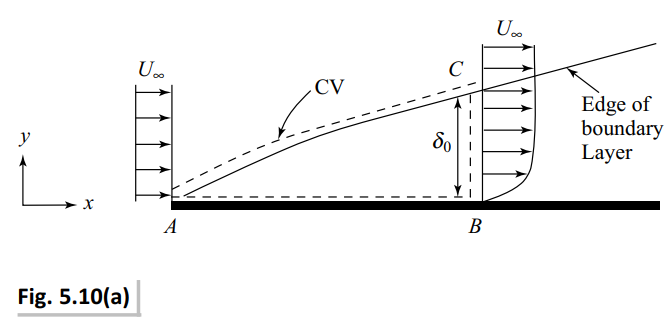
A fluid of constant density \rho flows over a stationary flat plate. The relative velocity between the solid boundary and the fluid in contact with that is zero (no-slip boundary condition). The flow domain may be conceptually divided into two parts, viz., a region adhering to the plate in which viscous effects are important and an outer region where viscous effects are negligible. The imaginary line that demarcates these two regions is the edge of the so called boundary layer, as shown in the Fig. 5.10. Incipient free stream velocity on the plate is U_{\infty}. The velocity distribution within the boundary layer is approximated by \frac{u}{U_{\infty}}=2 \frac{y}{\delta}-\left(\frac{y}{\delta}\right)^{2}. The boundary layer thickness at location B is \delta_{0} . The plate width perpendicular to the plane of the figure is w. Find the net drag force exerted by the plate on the fluid over the length L.

Learn more on how we answer questions.
Choose a fixed CV as shown by the dashed line in Fig. 5.10 (a).
0=0+\rho \int_{0}^{\delta_{0}} u d y w+\dot{m}_{A C}\dot{m}_{A C}=-\rho \int_{0}^{\delta_{0}} u d y w
Applying the x component of the linear momentum conservation equation, we have
F_{x}=0+\int_{0}^{\delta_{0}} \rho u u w d y+u_{A C} \cdot \dot{m}_{A C}
F_{x}=\rho w\left[\int_{0}^{\delta_{0}} u^{2} d y-U_{\infty} \int_{0}^{\delta_{0}} u d y\right]=\rho w \int_{0}^{\delta_{0}}\left(u^{2}-u U_{\infty}\right) d y (5.23)
Substituting \frac{u}{U_{\infty}}=2 \frac{y}{\delta}-\left(\frac{y}{\delta}\right)^{2} into Eq. (5.23), and letting \eta=\frac{y}{\delta}, we obtain
F_{x}=2 \rho w\left[U_{\infty}^{2} \delta_{0} \int_{0}^{1}\left(\eta-\frac{1}{2} \eta^{2}\right)^{2} d \eta-U_{\infty}^{2} \delta_{0} \int_{0}^{1}\left(\eta-\frac{1}{2} \eta^{2}\right) d \eta\right]=2 \rho w U_{\infty}^{2} \delta_{0}\left[\int_{0}^{1}\left(\eta^{2}+\frac{1}{4} \eta^{4}-\eta^{3}\right) d \eta-\int_{0}^{1}\left(\eta-\frac{1}{2} \eta^{2}\right) d \eta\right]
=2 \rho w U_{\infty}^{2} \delta_{0}\left[\frac{3}{2} \frac{\eta^{3}}{3}-\frac{\eta^{2}}{2}-\frac{\eta^{4}}{4}+\frac{1}{4} \frac{\eta^{5}}{5}\right]_{0}^{1}
=2 \rho w U_{\infty}^{2} \delta_{0}\left[\frac{3}{2} \frac{1}{3}-\frac{1}{2}-\frac{1}{4}+\frac{1}{4} \frac{1}{5}\right]
=-\frac{2}{5} \rho w U_{\infty}^{2} \delta_{0}
This is the force exerted by the plate on the fluid. Note that the minus sign indicates a force along the negative x direction, i.e, the force tends to slow the fluid down (hence the name drag force). Also note that by Newton’s third law, the drag force exerted by the fluid on the plate will be \frac{2}{5} \rho w U_{\infty}^{2} \delta_{0} , which is a force along the positive x direction.
Alternative Choice of the Control Volume (CV)
The very fact that there is a flow across AC in Fig. 5.10(a) renders our calculations somewhat tedious, which may be simplified to some extent if we choose another reference line instead of AC such that the net flow across that new reference line is zero. Such a line may be chosen by considering the streamline passing through C (i.e., DC in Fig. 5.10(b)), since by definition there is no flow across a streamline. This motivates us to choose the CV as ABCD, as indicated in Fig. 5.10(b). Further, because of no penetration boundary condition at the plate (i.e., zero normal component of flow velocity at the wall), there is no flux across the surfaces A B. Thus fluxes flow out only across the surfaces AD and BC.
From conservation of mass for the CV, we get
0=0+\int_{A D} \rho(\vec{V} \cdot \hat{n}) d A+\int_{B C} \rho(\vec{V} \cdot \hat{n}) d Ai.e., 0=0+\rho \int_{0}^{h_{0}}\left(-U_{\infty}\right) w d y+\int_{0}^{\delta_{o}} \rho u w d y
i.e., U_{\infty} h_{0}=\int_{0}^{\delta_{0}} u d y (5.24)
Applying the x component of momentum conservation equation for the CV, we have
F_{x}=\int_{A D} \rho u(\vec{V} . \hat{n}) d A+\int_{B C} \rho u(\vec{V} . \hat{n}) d A=\rho \int_{0}^{h_{0}} U_{\infty}\left(-U_{\infty}\right) w d y+\rho \int_{0}^{\delta_{o}} u(u) w d y
=-\rho U_{\infty}^{2} w h_{0}+\rho w \int_{0}^{\delta_{0}} u^{2} d y
=-\rho U_{\infty} w \int_{0}^{\delta_{0}} u d y+\rho w \int_{0}^{\delta_{0}} u^{2} d y
(Substituting U_{\infty} h_{0} from Eq. (5.24))
Thus, F_{x}=\rho w\left[\int_{0}^{\delta_{0}} u^{2} d y-U_{\infty} \int_{0}^{\delta_{0}} u d y\right]
The remaining part of the solution is the same as that obtained by the previous method.