Question 9.3: A steel beam is supported and loaded as shown in Fig. 9.36. ...

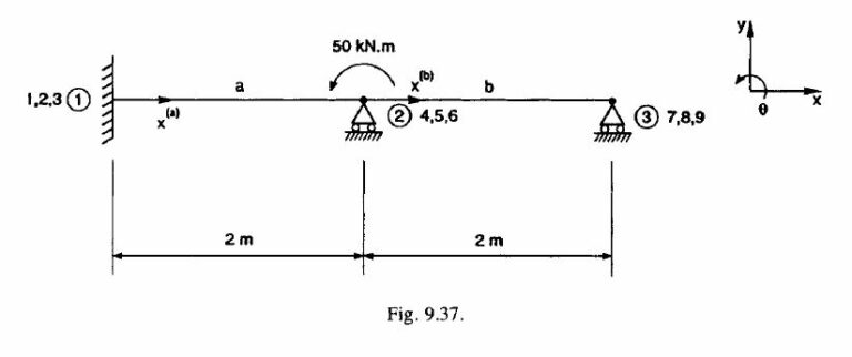
(a) Figure 9.37 shows suitable node, dof. and element labelling. Lack of symmetry prevents any advantage being taken to reduce the calculations. There are no redundant members. Employing two beam finite elements, (which is the least number in this case), both elements will have the same E/L, i.e,

(E/L)^{(a)}=(E/L)^{(b)}=E/L

However, the second moments of area will be different, such that

I^{(a)}=2I \text{ and } I^{(b)}=I

and will be the only difference between the two element stiffness matrices. With reference to §9.8 and in the absence of axial forces, each element stiffness matrix with respect to local coordinates is given as

[k^{(e)}]=(\frac{EI}{L} )^{(e)}\begin{bmatrix} 12/L^{2} & & \\ 6/L &4 & symmetric & \\ -12/L&-6/L&12/L^{2} & \\6/L &2&-6/L & 4\end{bmatrix}

The above local coordinate element stiffness matrix will, in this case, be identical to that with respect to global coordinates since the local and global axes coincide.

Substituting for both elements:

Element a

Recalling I^{(a)}=2I

[k^{(a)}]=(\frac{EI}{L} )\begin{bmatrix} 24/L^{2} & & \\ 12/L &8 & symmetric & \\ -24/L&-12/L&24/L^{2} & \\12/L &4&-12/L & 8\end{bmatrix}

Element b
Recalling I^{(b)} = I

[k^{(b)}]=(\frac{EI}{L} )\begin{bmatrix} 12/L^{2} & & \\6/L &4 & symmetric & \\ -12/L&-6/L&12/L^{2} & \\6/L &2&-6/L & 4\end{bmatrix}

The structural stiffness matrix can now be assembled. A dof. correspondence table can be used as an aid to assembly. However, observation of the relatively simple element connectivity, shows that the stiffness contributions for element a will occupy the upper left 4 × 4 locations, whilst those for element h will occupy the lower right 4 × 4 locations of the 6 × 6 structural stiffness matrix. The reduced structural stiffness matrix is due to the omission of axial terms, otherwise the matrix would have been of order 9 × 9. Hence, completing only those columns needed for the solution, gives

Corresponding to \upsilon _{1}=\theta _{1}=\upsilon _{2}=\upsilon _{3}=0 (by omitting axial terms it has already been taken that u_{1}=u _{2}=u_{3}=0), the partitioned equations reduce to

\begin{bmatrix} M_{2} \\ M_{3} \end{bmatrix} =\frac{EI}{L} \begin{bmatrix} 12 & 2 \\ 2 & 4 \end{bmatrix} \begin{bmatrix} \theta _{2} \\ \theta _{3} \end{bmatrix}    i.e \left\{P_{\alpha }\right\} =[K_{\alpha \alpha }] \left\{P_{\alpha }\right\}

Inverting [K_{\alpha \alpha}] to enable a solution for the displacements from \left\{P_{\alpha }\right\} =[K_{\alpha \alpha }]^{-1} \left\{P_{\alpha }\right\}

where adj [K_{\alpha \alpha }]=\frac{EI}{L}\begin{bmatrix} 4 & -2 \\ -2 & 12 \end{bmatrix}  and det   [K_{\alpha \alpha }]=44(EI/L)^{2}

then [K_{\alpha \alpha }]^{-1}=\frac{L}{44EI} \begin{bmatrix}4& -2 \\ -2 & 12\end{bmatrix}  check  \frac{L}{44 EI} \begin{bmatrix}4& -2 \\ -2 & 12\end{bmatrix} \frac{EI}{L} \begin{bmatrix}12& 2 \\ 2 &4\end{bmatrix} =[I]

The required displacements are found from

\left\{P_{\alpha }\right\} =[K_{\alpha \alpha }]^{-1} \left\{P_{\alpha }\right\}

Substituting    \begin{bmatrix} \theta _{2} \\ \theta _{3} \end{bmatrix}=\frac{L}{44EI} \begin{bmatrix}4& -2 \\ -2 & 12\end{bmatrix} \begin{bmatrix} M_{2} \\ M_{3} \end{bmatrix}

The required nodal displacements are therefore \theta _{2}=0.26°  and  \theta _{3}=-0.13°
(b) With reference to §9.12, nodal reactions are obtained from

Substituting gives  \begin{bmatrix} Y_{1} \\ M_{} \\Y_{2} \\M_{2} \end{bmatrix} =\frac{EI}{L} \begin{bmatrix} 12/L & 0 \\4 & 0 \\ -6/L & 6/L \\ -6/L & -6/L \end{bmatrix} \begin{bmatrix} \theta _{2} \\ \theta _{3} \end{bmatrix}

The required nodal reactions are therefore Y _{1} = 27.27 \ kN, \ M_{1} = 18.18 \ kNm, \ Y_{2} = -20.45 \ kN and Y_{3} = -6.82 \ kN.
Representing these reactions together with the applied moment on a sketch of the deformed beam, Fig. 9.38, and considering force and moment equilibrium, gives

\sum{F_{y}} =(27.27-20.45-6.82) \ kN=0

\sum{M_{1}} =(18.18+50-20.45\times 2-6.82\times 4) \ kNm=0