Question 8.CS.2: UFSS Vehicle: Transient Design via Gain In this case study, ...
UFSS Vehicle: Transient Design via Gain
In this case study, we apply the root locus to the UFSS vehicle pitch control loop. The pitch control loop is shown with both rate and position feedback in Appendix A3. In the example that follows, we plot the root locus without the rate feedback and then with the rate feedback. We will see the stabilizing effect that rate feedback has upon the system.
Consider the block diagram of the pitch control loop for the UFSS vehicle shown in Appendix A3 (Johnson, 1980).
a. If K_{2} = 0 (no rate feedback), plot the root locus for the system as a function of pitch gain, K_{1} , and estimate the settling time and peak time of the closed-loop response with 20% overshoot.
b. Let K_{2} = K_{1} (add rate feedback) and repeat a.
Learn more on how we answer questions.
a. Letting K_{2} = 0, the open-loop transfer function is
G (s) H (s) = \frac{0.25 K_{1} (s + 0.435)}{(s + 1.23) (s + 2) (s² + 0.226s + 0.0169)} (8.74)
from which the root locus is plotted in Figure 8.30. Searching along the 20% overshoot line evaluated from Eq. (8.39), we find the dominant second-order poles to be −0.202 ±j 0.394 with a gain of K = 0.25K_{1} = 0.706, or K_{1} = 2.824.
11σ² − 26σ − 61 = 0 (8.39)
From the real part of the dominant pole, the settling time is estimated to be T_{s} = 4/0.202 = 19.8 seconds. From the imaginary part of the dominant pole, the peak time is estimated to be T_{p} = π/0.394 = 7.97 seconds. Since our estimates are based upon a second-order assumption, we now test our assumption by finding the third closed-loop pole location between −0.435 and −1.23 and the fourth closed-loop pole location between −2 and infinity. Searching each of these regions for a gain of K = 0.706, we find the third and fourth poles at −0.784 and −2.27, respectively. The third pole, at −0.784, may not be close enough to the zero at −0.435, and thus the system should be simulated. The fourth pole, at −2.27, is 11 times as far from the imaginary axis as the dominant poles and thus meets the requirement of at least five times the real part of the dominant poles.
A computer simulation of the step response for the system, which is shown in Figure 8.31, shows a 29% overshoot above a final value of 0.88, approximately 20-second settling time, and a peak time of approximately 7.5 seconds.
b. Adding rate feedback by letting K_{2} = K_{1} in the pitch control system shown in Appendix A3, we proceed to find the new open-loop transfer function. Pushing −K_{1} to the right past the summing junction, dividing the pitch rate sensor by −K_{1} , and combining the two resulting feedback paths obtaining (s + 1) give us the following open-loop transfer function:
G (s) H (s) = \frac{0.25K_{1} (s + 0.435) (s + 1) }{(s + 1.23)(s + 2)(s² + 0.226s + 0.0169)} (8.75)
Notice that the addition of rate feedback adds a zero to the open-loop transfer function. The resulting root locus is shown in Figure 8.32. Notice that this root locus, unlike the root locus in a, is stable for all values of gain, since the locus does not enter the right half of the s-plane for any value of positive gain, K = 0.25K_{1} . Also notice that the intersection with the 20% overshoot line is much farther from the imaginary axis than is the case without rate feedback, resulting in a faster response time for the system.
The root locus intersects the 20% overshoot line at −1.024 ±j1.998 with a gain of K = 0.25K_{1} = 5.17, or K_{1} = 20.68. Using the real and imaginary parts of the dominant pole location, the settling time is predicted to zzbe T_{s} = 4/1.024 = 3.9 seconds, and the peak time is estimated to be T_{p} = π/1.998 = 1.57 seconds. The new estimates show considerable improvement in the transient response as compared to the system without the rate feedback.
Now we test our second-order approximation by finding the location of the third and fourth poles between −0.435 and −1. Searching this region for a gain of K = 5.17, we locate the third and fourth poles at approximately −0.5 and −0.91. Since the zero at −1 is a zero of H(s), the student can verify that this zero is not a zero of the closed-loop transfer function. Thus, although there may be pole-zero cancellation between the closed-loop pole at −0.5 and the closed-loop zero at −0.435, there is no closed-loop zero to cancel the closed-loop pole at −0.91.² Our second-order approximation is not valid.
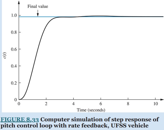
A computer simulation of the system with rate feedback is shown in Figure 8.33. Although the response shows that our second-order approximation is invalid, it still represents a considerable improvement in performance over the system without rate feedback; the percent overshoot is small, and the settling time is about 6 seconds instead of about 20 seconds.
CHALLENGE:
You are now given a problem to test your knowledge of this chapter’s objectives. For the UFSS vehicle (Johnson, 1980) heading control system shown in Appendix A3, and introduced in the case study challenge in Chapter 5, do the following:
a. Let K_{2} = K_{1} and find the value of K_{1} that yields 10% overshoot.
b. Repeat, using MATLAB.