Question 10.3.1: Let f(x) = {0, −L < x < 0, L , 0 < x < L , (5) a......

Three periods of the graph of y = f(x) are shown in Figure 10.3.2; it extends periodically to infinity in both directions. It can be thought of as representing a square wave. The interval [−L , L] can be partitioned into the two open subintervals (−L , 0) and (0, L). In (0, L), f(x) = L and f′(x) = 0. Clearly, both f and f ′ are continuous and furthermore have limits as x → 0 from the right and as x → L from the left. The situation in (−L , 0) is similar. Consequently, both f and f ′ are piecewise continuous on [−L , L) , so f satisfies the conditions of Theorem 10.3.1. If the coefficients a_{m} and b_{m} are computed from equations (2)

a_{m}=\frac{1}{L}\int_{-L}^{L}f(x)\cos\Bigl(\frac{m\pi x}{L}\Bigr)d x,\quad m=0,1,2,\dots\ ; (2)

and (3),

b_{m}=\frac{1}{L}\int_{-L}^{L}f(x)\sin\Bigl(\frac{m\pi x}{L}\Bigr)d x,\quad m=1,2,\,\ldots\,. (3)

the convergence of the resulting Fourier series to f(x) is ensured at all points where f is continuous. Note that the values of the Fourier coefficients a_{m} and b_{m} are the same regardless of the definition of f at its points of discontinuity. This is true because the value of an integral is unaffected by changing the value of the integrand at a finite number of points. From equation (2),

a_{0}=\frac{1}{L}\int_{-L}^{L}f(x)d x=\int_{0}^{L}1d x=L

and

a_{m}={\frac{1}{L}}\int_{-L}^{L}f(x)\cos\Bigl({\frac{m\pi x}{L}}\Bigr)d x=\int_{0}^{L}\cos\Bigl({\frac{m\pi x}{L}}\Bigr)d x\\ ={\frac{L}{m\pi}}(\sin(m\pi)-0)=0,\quad m\neq0.

Similarly, from equation (3),

b_{m}={\frac{1}{L}}\int_{-L}^{L}f(x)\sin\Bigl({\frac{m\pi x}{L}}\Bigr)d x=\int_{0}^{L}\sin\Bigl({\frac{m\pi x}{L}}\Bigr)d x\\ ={\frac{L}{m\pi}}(1-\cos(m\pi))=\begin{cases}0, & \text{m even;} \\\frac{2L}{mx}, & \text{m odd.}\end{cases}

Hence

f(x)={\frac{L}{2}}+{\frac{2L}{\pi}}\left(\sin\left({\frac{\pi x}{L}}\right)+{\frac{1}{3}}\sin\left({\frac{3\pi x}{L}}\right)+{\frac{1}{5}}\sin\left({\frac{5\pi x}{L}}\right)+\cdots\right)\\ ={\frac{L}{2}}+{\frac{2L}{\pi}}\sum_{m=1,3,5,\ldots}^{\infty}{\frac{1}{m}}\sin\left({\frac{m\pi x}{L}}\right)\\={\frac{L}{2}}+{\frac{2L}{\pi}}\sum_{n=1}^{\infty}{\frac{1}{2n-1}}\sin\left({\frac{(2n-1)\pi x}{L}}\right). (6)

At the points x = 0, ±nL, where the function f in the example is not continuous, all terms in the series after the first vanish and the sum is L/2. This is the mean value of the limits from the right and left, as it should be. Thus we might as well define f at these points to have the value L/2.

If we choose to define it otherwise, the series still gives the value L/2 at these points, since all of the preceding calculations remain valid. The series simply does not converge to the function at those points unless f is defined to have the value L/2. This illustrates the possibility that the Fourier series corresponding to a function may not converge to it at points of discontinuity unless the function is suitably defined at such points.

The manner in which the partial sums

s_{n}(x)={\frac{L}{2}}+{\frac{2L}{\pi}}\left(\sin\left({\frac{\pi x}{L}}\right)+\cdot\cdot\cdot+{\frac{1}{2n-1}}\sin\left({\frac{(2n-1)\pi x}{L}}\right)\right),\quad n=1,2, \dots

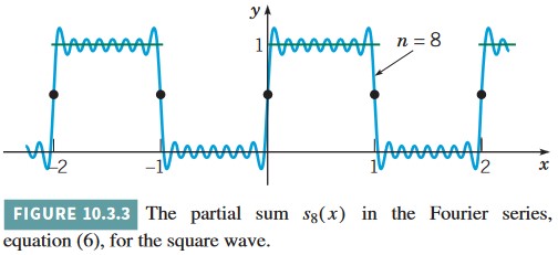
of the Fourier series (6) converge to f(x) is indicated in Figure 10.3.3, where L has been chosen to be 1 and the graph of s_{8}(x) is plotted. The figure suggests that at points where f is continuous, the partial sums do approach f(x) as n increases. However, in the neighborhood of points of discontinuity, such as x = 0 and x = L, the partial sums do not converge smoothly to the mean value. Instead, they tend to overshoot the mark at each end of the jump, as though they cannot quite accommodate themselves to the sharp turn required at this point. This behavior is typical of Fourier series at points of discontinuity and is known as the Gibbs^{5} phenomenon.

Additional insight is attained by considering the error e_{n}(x) = f(x) − s_{n}(x). Figure 10.3.4 shows a plot of |e_{n}(x)| versus x for n = 8 and for L = 1. The least upper bound of |e_{8}(x)| is 0.5 and is approached as x → 0 and as x → 1. As n increases, the error decreases in the interior of the interval [where f(x) is continuous], but the least upper bound does not diminish with increasing n. Thus we cannot uniformly reduce the error throughout the interval by increasing the number of terms.

Figures 10.3.3 and 10.3.4 also show that the series in this example converges more slowly than the one in Example 1 in Section 10.2. This is due to the fact that the coefficients in the series (6) are proportional only to 1/(2n − 1).

^{5}The Gibbs phenomenon is named after Josiah Willard Gibbs (1839-1903), who is better known for his work on vector analysis and statistical mechanics. Gibbs was professor of mathematical physics at Yale and one of the first American scientists to achieve an international reputation. The Gibbs phenomenon is discussed in more detail by Carslaw (Chapter 9).