Question 6.EC.2: Magnetic Braking on An Incl ined Plane Introduction When a......
Magnetic Braking on An Incl ined Plane
Introduction
When a magnet moves near a non-magnetic conductor such as copper and aluminum, it experiences a dissipative force called magnetic braking force. In this experiment we will investigate the nature of this force.
The magnetic braking force depends on:
– the strength of the magnet, determined by its magnetic moment (μ) ;
– the conductivity of the conductor (σ_c);
– the size and geometry of both magnet and the conductor;
– the distance between the magnet and conducting surface (d); and
– the velocity of the magnet (v) relative to the conductor.
In this experiment we will investigate the magnetic braking force dependencies on the velocity (v) and the conductor-magnet distance (d). This force can be written empirically as:
F_{\mathrm{MB}}=-\,k_{0}\,d^{p}v^{n}, (1)
where
k_{0} is an arbitrary constant that depends on μ, σ_c and geometry of the conductor and magnet which is fixed in this experiment.
d is the distance between the center of magnet to the conductor surface.
v is the velocity of the magnet.
p and n are the power factors to be determined in this experiment.
Experiment
In this experiment error analysis is required.
Apparatus
(1) Doughnut-shaped Neodymium Iron Boron magnet.
Thickness: t_{M} = (6.3 ± o. 1)mm
Outer diameter: d_{M} = (25.4 ± O. 1)mm
The poles are on the flat faces as shown:
(2) Aluminum bar (2 pieces).
(3) Acrylic plate for the inclined plane with a linear track for the magnet to roll.
(4) Plastic stand.
(5) Digital stop watch.
(6) Ruler.
(7) Graphic papers (10 pieces).
Additional infonnation:
Local gravitational acceleration: g = 9.8 m/s² •
Mass of the magnet: m = (21. 5±0. 5) gram.
North-South direction is indicated on the table.
You can read the operation manual of the stopwatch.
This problem is divided into two sections:
(A) Setup and introduction.
(B) Investigation of the magnetic braking force.
Questions
Please provide sufficient diagrams in your answers so that your work can be understood clearly.
(A) Setup
Roll down the magnet along the track as shown. Choose a reasonably small inclination angle so that it does not roll too fast.
(1) As the magnet is very strong, it may experience significant torque due to interaction with earth’s magnetic field. It will twist the magnet as it rolls down and may cause significant friction with the track. What will you do to minimize this torque? Explain it using diagram(s).
Place the two aluminum bars as shown m Fig. 6 – 20 with distance approximately d = 5 mm. Remember that the distance d is to the center of the magnet as shown in the inset of Fig. 6 – 20.
Again release the magnet and let it roll. You should observe that the magnet would roll down much slower compared to the previous observation due to magnetic braking force.
(2) Provide diagram(s) of field lines and forces to explain the mechanism of magnetic braking.
(B) Investigation of the magnetic braking force
The experimental setup remains the same as shown in Fig. 6 – 20. with the same magnet-conductor distance approximately d = 5 mm (about 2 mm gap between magnet and conductor on each side) .
(1) Keeping the distance d fixed, investigate the dependence of magnetic braking force on velocity (v). Determine the exponent n of the speed dependence factor in Equation (1). Provide appropriate graph to explain your result.
Now vary the conductor-magnet distance (d) on both left and right.
Choose a fixed and reasonably small inclination angle.
(2) Investigate the dependence of the magnetic braking force on conductor-magnet distance (d). Determine the exponent p of the distance dependence factor in Equation (1). Provide appropriate graph to explain your result.

Learn more on how we answer questions.
(A) Setup and Introduction
( 1) To minimize the torque due to interaction of the magnet and the earth’s magnetic field we have to set the orientation of the inclined plane so that the magnet will roll down with the poles aligned to the North-South direction as shown.
Answer with some vector analysis:
Consider a point A on the conductor. As the magnet moves, its magnetic field sweeps the conductor inducing electric field and causing current flow due to Faraday’s law, whose direction can be determined using Lenz’s law. Let us choose an arbitrary loop as shown. At point A, the magnetic field and the current will cause Lorentz force F_{M-C} pointing at x+ direction. This force is acting on the electrons in the conductor.
On the other hand, due to Newtons’ Third law there is reaction force F_{M-C} with the same magnitude but with opposite direction acting on the magnet, which is the magnetic braking force.
(B) Investigation of the magnetic braking force
(1) Determination of the power factor n: Dependence of the magnetic braking force with the velocity.
In this experiment the student has to be aware that the magnet should reach the terminal velocity first before start the timing. From observation we can see that the magnet reaches terminal velocity almost immediately.
To make sure we let the magnet travels first for about 5 cm before we start measuring the time. Here we use 5 = 250 mm from start to finish to obtain speed:v={\frac{s}{t}}.
The angle of inclination is varied to take several data. Given l = 425 mm, we measure h where \sin\theta={\frac{h}{l}}.
Because the magnet-conductor distance is kept constant ( d ≈ 5 mm) , the magnetic braking force only depends on the velocity of the magnet, so we can simplify
F_{\mathrm{MB}}=-\,k_{0}d^{p}v^{n}=-\,k_{1}\,v^{n},where k_{1}\,=\,k_{\mathrm{0}}d^{p} is constant in this experiment.
When the magnet reaches the terminal velocity then the total torque should be zero. The equation of the motion at the contact point C will be:
\sum{\tau c}=0,m\mathrm{g}\sin\theta R+F_{\mathrm{MB}}R=0\,,
m g\sin\theta-k_{1}v^{n}=0,
\sin\theta={\frac{k_{1}}{m g}}v^{n}.
To calculate the power factor n:
\mathrm{ln}\sin\theta=\mathrm{ln}\bigl(\frac{k_{1}}{m g}\bigr)+n\mathrm{ln}(v).The experimental data:
Table 1.
Note:
• Column in bold are the data directly taken from the experiment.
• Typical error for h measurement is shown in the first row: h = (23 ± 5)mm. Similar error applies for the rest of h data.
• Data \bar t are the average data taken from 3 to 5 measurement. Even though standard deviation error is quite small ( ± o. 1 s), the error should be dominated by response delay of the observer in pressing the stopwatch.
Widely accepted value for human eye response is 0.25 s, in this experiment we choose more conservative value ( ± 0.5 s).
Using linear regression method or graphical method as shown in Fig. 6 -22 one can determine n from the slope
n=0.96,
whose result is very close to the theoretical value of n = 1. From the data shown in Fig. 6 – 16 Cas well as the coefficient of correlation r = O. 9995) , it can be shown that this experiment is very good in demonstrating the linear velocity dependence of the magnetic braking force. This result has been repeated and verified by three independent persons and apparatus setups.
Error estimate of n
Instead of laboring on detailed error propagation analysis that could be very time consuming, in Olympiad context one can make the error estimate as follows:
The typical error of the data points in Fig. 6 – 22 can be obtained from the central data:
\ln(\sin\theta)=-1.8\pm0.075\,,
whose errors propagated from the uncertainties in h and t.
The power factor n can be obtained from the slope of Fig. 6 – 22:
n={\frac{\Delta y}{\Delta x}}where y=\ln(\sin\theta){\mathrm{~and}}\,x=\ln\upsilon.
From the data in Fig. 6 – 22, we have: Δx = 2. 1 and Δy = 2. 0, and the typical errors:\delta x = 0.075 and \delta y = 0.075.
So the error estimate for n:
\frac{\Delta n}{n}=\sqrt{\left(\frac{\delta x}{\Delta x}\right)^{2}+\left(\frac{\delta y}{\Delta y}\right)^{2}}\,=\sqrt{\left(\frac{0.075}{2.1}\right)^{2}+\left(\frac{0.075}{2.0}\right)^{2}}\,=0.05,Δn = O. 05n = O. 048.
So we can conclude the result of our experiment is
n = O. 96±0. 05,
(2) Determination of the power factor P: Dependence of the magnetic braking force with the magnet-conductor distance.
In this experiment we use one value of inclination angle, h = 50 mm (l =425 mm) so that \theta=\arcsin\!\,\!\left({\frac{h}{l}}\right)=6.8^{\circ}.. Distance travelled remains:
s =250 mm, and the timing is done after the magnet travel first for about 5 cm as before.
The equation of motion, similar to previous section:
mg~\mathrm{sin}\,\theta R+F_{MB}R=0\,,
m g\sin\theta-k_{0}d^{p}v^{n}=0,
v^{-n}=\frac{k_{0}}{m g\sin\theta}d^{p}\,,
-\,n\ln v=\ln\Bigl({\frac{k_{0}}{m g\sin\theta}}\Bigr)+p\ln d.
Here again p can be obtained using linear regression or graphical method where we use the previously obtained value: n = 0.96 ± 0.05.
The experimental data:
Table 2.
Note:
Distance d is measured from the center of the magnet.
From linear regression calculation we have
p =-2.16.
So the magnetic braking force is very sensitive with the magnet – conductor distance d in which the relationship is almost inversely quadratic. In brief, the further the magnet from the conductor the weaker the magnetic braking force becomes. This result has been repeated and verified by three independent persons and apparatus setups.
Error estimate of p
Similar to previous section, we use the central data shown in Fig. 6 – 24.
\ln d=2.01\pm0.105,-\,n\mathrm{ln}(v)=-\,3.76\pm0.095.
The power factor p can be obtained from the slope of line in di Fig. 6 – 24.
\rho={\frac{\Delta y}{\Delta x}} where y =-n ln v and x = ln d.
For the data shown in Fig. 6 – 24, we obtain: Δx = 0.94 dan Δy = 2.01, with typical error: \delta xx = 0.105 and \delta xy = 0.095.
So the error estimate for p:
\frac{\Delta p}{\rho}=\sqrt{\left(\frac{\delta x}{\Delta x}\right)^{2}+\left(\frac{\delta y}{\Delta y}\right)^{2}}=\sqrt{\left(\frac{0.105}{0.94}\right)^{2}+\left(\frac{0.095}{2.01}\right)^{2}}=0.12,Δp = 0. 12p = 0.26.
So we can conclude the result of our experiment is
P =-2. 2 ± 0.3.
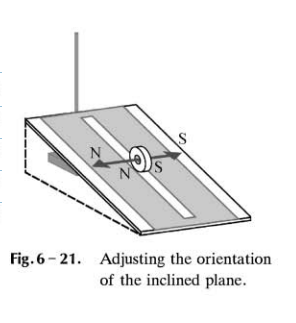


Table 1. Experimental data for power factor n determination.
| H(mm) | \overline t(\mathbf{s}) | sin θ | v(mm/s) | In(v) | In(sin θ) |
| 23 ±0. 5 | 22. 98 ± 0. 005 | 0.054 | 10.88 | 2.39 | -2.92 |
| 40 | 12. 78 | 0.094 | 19.56 | 2.97 | -2.36 |
| 50 | 10.17 | 0.118 | 24. 58 | 3. 20 | -2.14 |
| 60 | 8.62 | 0.141 | 29. 00 | 3.37 | -1. 96 |
| 70 | 6.96 | 0.165 | 35. 92 | 3. 58 | -1. 80 |
cont.
| H(mm) | \overline t(\mathbf{s}) | sin θ | v(mm/s) | In(v) | In(sin θ) |
| 80 | 6.09 | 0.188 | 41.05 | 3.71 | -1.67 |
| 91 | 5.48 | 0.214 | 45.62 | 3.82 | -1.54 |
| 101 | 5.05 | 0.238 | 49. 50 | 3. 90 | -1.44 |
| 111 | 4.57 | 0.261 | 54. 70 | 4. 00 | -1.34 |
| 120 | 4.17 | 0.282 | 59.95 | 4.09 | -1.26 |
| 130 | 3.72 | 0.306 | 67. 20 | 4.21 | -1.18 |
| 150 | 3.25 | 0.353 | 76.92 | 4.34 | -1.04 |
| 170 | 2.81 | 0. 400 | 88.97 | 4.49 | -0.92 |
Table 2. Experimental data for power factor p determination.
| d(mm) | t(s) | v(mm/s) | -nlnv | ln d |
| 4. 5±0. 5 | 13.53 ± 0.005 | 18.48 | -2. 80 | 1. 50 |
| 5.5 | 9. 60 | 26.04 | -3.13 | 1. 70 |
| 6.5 | 6. 70 | 37.31 | -3.47 | 1. 87 |
| 7.5 | 4.99 | 50. 10 | -3.76 | 2.01 |
| 8.5 | 3.47 | 72.05 | -4.11 | 2. 14 |
| 9.5 | 2.87 | 87.11 | -4.29 | 2.25 |
| 10.5 | 2.14 | 116.82 | -4.57 | 2.35 |
| 11.5 | 1.66 | 150. 60 | -4.81 | 2.44 |