Question 2.3: (a) Derive an expression for the displacement response, z, w......
(a) Derive an expression for the displacement response, z, when a step force of magnitude P is applied to the single-DOF system shown in Fig. 2.10. Assume that the damping is less than critical, and that the initial conditions are z = \dot {z} = 0 at t = 0.
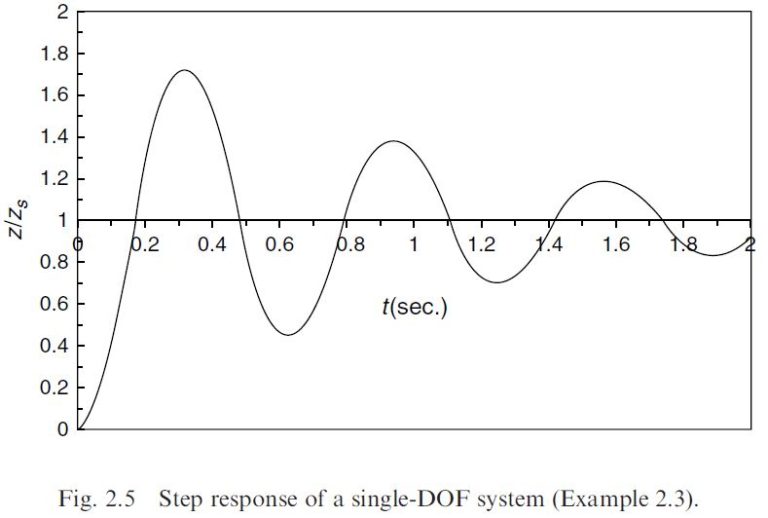
(b) Plot the displacement, z, in non-dimensional form, as a multiple of the static displacement for the same load, x_{s} = P/k, with the non-dimensional viscous damping coefficient, \gamma, equal to 0.1, and the undamped natural frequency, \omega_{n}, equal to 10 rad/s.
Learn more on how do we answer questions.
Part (a) :
In this case the equation to be solved is
m \ddot{z} +c\dot{z} + kz = P (A)
Equation (A) can be written in a form similar to Eq. (2.20),
\ddot{z} + 2\gamma \omega _{n}\dot{z} + \omega ^{2}_{n} z = 0 (2.20)
sometimes known as the ‘standard form’:
\ddot{z} + 2\gamma \omega _{n}\dot{z} + \omega ^{2}_{n} z = P / m (B)
Since \gamma <1, the complementary function z = e^{-\gamma \omega _{n}t}(A \cos \omega _{d}t + B \sin \omega _{d}t ), Eq. (2.28), is appropriate. For the particular integral, from Table 2.1, we try z = C, which makes \dot{z} = 0 and \ddot{z} = 0. Substituting these into Eq. (B) gives C=P/m\omega ^{2}_{n}, so the complete solution is
z = e^{-\gamma \omega _{n}t}(A \cos \omega _{d} t + B \sin \omega _{d} t ) +P/(m \omega ^{2}_{n} ) (C)
Differentiating
\dot{z} = e^{-\gamma \omega _{n}t}[(B\omega _{d} – A\gamma \omega _{n})\cos \omega _{d}t – (A\omega _{d} + B\gamma \omega _{n}) \sin \omega _{d}t] (D)
Inserting the initial conditions z = 0 and \dot{z} = 0 at t = 0 into Eqs (C) and(D), and solving for the constants A and B gives, using Eqs (2.16) and (2.26),
\omega _{n} = \sqrt{\frac{k}{m} } (2.16)
\omega _{d} = \omega _{n}\sqrt{(1-\gamma ^{2})} (2.26)
A = -P/(m\omega ^{2}_{n} ) = – P/k (E)
and
B = – P\gamma \omega _{n} / (m\omega ^{2}_{n} \omega _{d}) = – \frac{P\gamma }{k\sqrt{1-\gamma ^{2}} } (F)
Inserting Eqs (E) and (F) into Eq. (C), gives the solution:
z = \frac{P}{k}\left[1- e^{-\gamma \omega _{n}t} \left(\cos \omega _{d}t + \frac{\gamma }{\sqrt{(1-\gamma ^{2})} } \sin \omega _{d}t \right) \right] (G)
Part (b) :
Now the displacement of the system when a static load, equal in magnitude to P, is applied, is z_{s}, say, where z_{s} = P/k. Dividing both sides of Eq. (G) by z_{s}, we have a non-dimensional version:
\frac{z}{z_{s}} = 1- e^{-\gamma \omega _{n}t} \left(\cos \omega _{d}t + \frac{\gamma }{\sqrt{1-\gamma ^{2}} } \sin \omega _{d}t \right) (H)
This is plotted in Fig. 2.5, with \gamma = 0.1 and \omega _{n} = 10. It is seen that the displacement approaches twice the static value, before settling at the static value.
| Table 2.1 | |
| Form of F | Form of the particular integral |
| F = a constant | z = C |
| F = At | z = Ct + D |
| F = At² | z = Ct² + Dt + E |
| F = A sin ωt or A cos ωt | z = C cos ωt + D sin ωt |