Question 10.6.3: A PI control system is shown in Figure 10.6.2. Suppose the p......
A PI control system is shown in Figure 10.6.2. Suppose the plant has the parameter values I = 5 and c = 2. The dominant time constant is specified to be 0.5 s.
a. Compute the required values for K_P and K_I for each of the following three cases:
(1) ζ = 0.707, (2) ζ = 1, and (3) The secondary time constant must be 0.05 s.
Evaluate the steady-state command error and the steady-state disturbance error for each case given that both the command input ω_r (t) and the disturbance T_d (t) are unit-step functions.
b. Plot the output response ω(t) and the actuator response T (t) for each case, given that the command input ω_r (t) is a unit-step function and the disturbance T_d (t) is zero.
c. Evaluate the steady-state command error for each case given that the command input ω_r (t) is a unit-ramp function and the disturbance T_d (t) is zero.
d. Evaluate the frequency response characteristics of the disturbance transfer function.

Learn more on how do we answer questions.
From the block diagram we obtain the following output, error, and actuator equations.
\Omega(s)=\frac{K_P s + K_I}{5 s^2 + \left(2 + K_P\right) s + K_I} \Omega_r(s)-\frac{s}{5 s^2 + \left(2+K_P\right) s + K_I} T_d(s) (1)
E(s)=\frac{5 s^2 + 2 s}{5 s^2 + \left(2+K_P\right) s + K_I} \Omega_r(s)+\frac{s}{5 s^2 + \left(2+K_P\right) s + K_I} T_d(s) (2)
T(s)=\frac{\left(K_P s + K_I\right)(5 s+2)}{5 s^2+\left(2 + K_P\right) s + K_I} \Omega_r(s)+\frac{K_P s + K_I}{5 s^2 + \left(2 + K_P\right) s + K_I} T_d(s) (3)
The characteristic equation is
5 s^2+\left(2+K_P\right) s+K_I=0 (4)
and its roots are
s=\frac{-\left(2 + K_P\right) \pm \sqrt{\left(2 + K_P\right)^2 – 20 K_I}}{10}
The Routh-Hurwitz condition shows the system is stable if 2 + K_P > 0 and K_I > 0. Applying the final value theorem to the error equation (2) with Ω_r (s) = 1/s and T_d (s) = 0 gives
e_{s s}=\underset{s \rightarrow 0}{lim} s E(s)=\underset{s \rightarrow 0}{lim} s \frac{5 s^2 + 2 s}{5 s^2 + \left(2 + K_P\right) s + K_I} \frac{1}{s}=0
if the system is stable. Thus the system has zero command error for a step command.
Applying the final value theorem to the error equation (2) with Ω_r (s) = 0 and T_d (s) = 1/s gives
e_{s s}=\underset{s \rightarrow 0}{lim} s E(s)=\underset{s \rightarrow 0}{lim} s \frac{s}{5 s^2 + \left(2 + K_P\right) s + K_I} \frac{1}{s}=0
if the system is stable. Thus the system has zero disturbance error for a step disturbance.
The damping ratio is
\zeta=\frac{2 + K_P}{2 \sqrt{5 K_I}}
The presence of K_I enables the damping ratio to be selected without fixing the value of the dominant time constant. For example, if the system is underdamped or critically damped, the time constant is
\tau=\frac{10}{2 + K_P} (if ζ ≤ 1)
The gain K_P can be picked to obtain the desired time constant, while K_I is used to set the damping ratio. Complete description of the transient response requires the numerator dynamics present in the transfer functions to be accounted for.
a. Case 1: If ζ < 1, the real part of the roots is −(2+ K_P )/10, and thus the time constant is
\tau=\frac{10}{2 + K_P}=0.5 sec
which gives K_P = 18. The damping ratio of equation (4) is
\zeta=\frac{2 + K_P}{2 \sqrt{5 K_I}}=0.707
Using K_P = 18 and squaring both sides gives
\frac{20^2}{4\left(5 K_I\right)}=(0.707)^2=0.5
Solve for K_I to obtain K_I = 40.
Case 2: If ζ = 1, the roots of equation (4) are both equal to −(2 + K_P )/10, and thus the time constant is
\tau=\frac{10}{2 + K_P}=0.5
which gives K_P = 18. Using this value in the damping ratio of equation (4), we have
\zeta=\frac{2 + K_P}{2 \sqrt{5 K_I}}=\frac{10}{\sqrt{5 K_I}}=1
Squaring both sides gives
\frac{10^2}{5 K_I}=1
Solve for K_I to obtain K_I = 20.
Case 3: Since ζ > 1 in this case, the expressions for the time constants of equation (4) are too complicated to be useful. The easier approach is to express the desired characteristic equation in factored form. The desired time constants are 0.5 s and 0.05 s, which correspond to the roots s = −2 and s = −20. The desired characteristic equation may thus be expressed as
(s + 2)(s + 20) = s² + 22s + 40 = 0
To compare this with equation (4) we must multiply by 5 to obtain
5s² + 110s + 200 = 0
Comparison of this with equation (4) shows that K_I = 200 and 2 + K_P = 110, which gives K_P = 108. These gain values give a damping ratio of ζ = 110/2 \sqrt{1000} = 1.74.
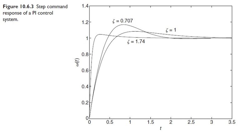
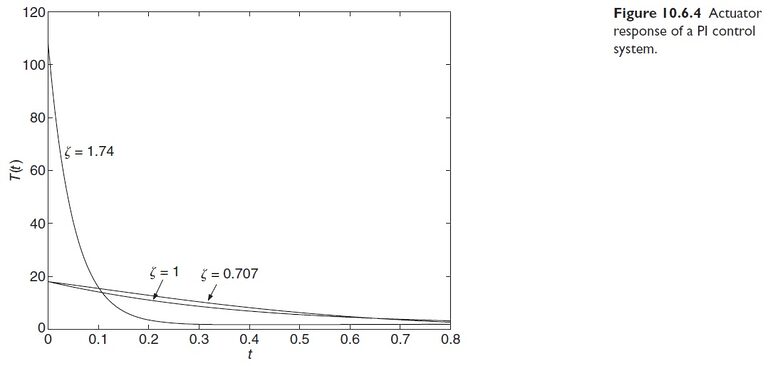
b. The plots can be easily obtained with MATLAB using the \boxed{tf} and \boxed{step} functions applied to equations (1) and (3). The plots are shown in Figures 10.6.3 and 10.6.4. The design having the shortest rise time and shortest settling time is case 3 with ζ = 1.74. It also has the smallest overshoot. That case, however, requires the greatest output from the actuator, as seen in Figure 10.6.4. The maximum torque values for each case are 18, 18, and 108, respectively.
c. Applying the final value theorem to the error equation (2) with Ω_r (s) = 1/s² and T_d (s) = 0 gives
e_{s s}=\underset{s \rightarrow 0}{lim} s E(s)=\underset{s \rightarrow 0}{lim} s \frac{5 s^2 + 2 s}{5 s^2 + \left(2 + K_P\right) s + K_I} \frac{1}{s^2}=\frac{2}{K_I}
Thus the steady-state ramp command error is nonzero and is different for each of the three cases. It is the smallest for case 3 because that case has the largest value of K_I .
The following table summarizes the results.
d. The disturbance frequency response plot for each case is shown in Figure 10.6.5.
The bandwidths for each case are slightly different, but the disturbance amplification for case 3 is much smaller than for the other two cases. The peak values are −26.02, −26.02, and −40.85 dB, respectively. These correspond to magnitude ratios of 0.05, 0.05, and 0.0091.
| Ramp command error | Maximum torque | ζ | K_I | K_P | Case |
| 0.05 | 18 | 0.707 | 40 | 18 | 1 |
| 0.1 | 18 | 1 | 20 | 18 | 2 |
| 0.005 | 108 | 1.74 | 200 | 108 | 3 |