Question 5.6: A three-phase, 75-MVA, 13.8-kV synchronous generator with sa......
A three-phase, 75-MVA, 13.8-kV synchronous generator with saturated synchronous reactance X_s = 1.35 per unit and unsaturated synchronous reactance X_{s,u} = 1.56 per unit is connected to an external system with equivalent reactance X_{EQ} = 0.23 per unit and voltage V_{EQ} = 1.0 per unit, both on the generator base. It achieves rated open-circuit voltage at a field current of 297 amperes.
a. Find the maximum power P_{max} (in MW and per unit) that can be supplied to the external system if the internal voltage of the generator is held equal to 1.0 per unit.
b. Using MATLAB,^† plot the terminal voltage of the generator as the generator output is varied from zero to P_{max} under the conditions of part (a).
c. Now assume that the generator is equipped with an automatic voltage regulator which controls the field current to maintain constant terminal voltage. If the generator is loaded to its rated value, calculate the corresponding power angle, per-unit internal voltage, and field current. Using MATLAB, plot per-unit E_{af} as a function of per-unit power.
Learn more on how do we answer questions.
a. From Eq. 5.47
P=\frac{E_{af}V_{EQ}}{X_s + X_{EQ}} \sin δ (5.47)
P_{max}=\frac{E_{af}V_{EQ}}{X_s + X_{EQ}}
Note that although this is a three-phase generator, no factor of 3 is required because we are working in per unit.
Because the machine is operating with a terminal voltage near its rated value, we should express P_{max} in terms of the saturated synchronous reactance. Thus
P_{max}=\frac{1}{1.35 + 0.23} = 0.633 per unit = 47.5 MW
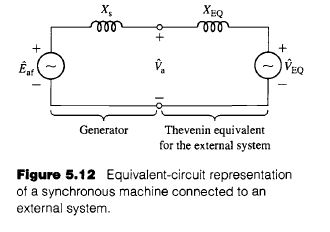
b. From Fig 5.12, the generator terminal current is given by
\hat{I}_a =\frac{\hat{E}_{af} – \hat{V}_{EQ}}{j(X_s +X_{EQ})}= \frac{E_{af} e^{jδ}- V_{EQ}}{ j(X_s +X_{EQ})}=\frac{e^{jδ}-1.0}{j1.58}
The generator terminal voltage is then given by
\hat{V}_a=\hat{V}_{EQ}+ jX_{EQ}\hat{I}_a=1.0+\frac{.23}{1.58}(e^{jδ}-1.0)
Figure 5.13a is the desired MATLAB plot. The terminal voltage can be seen to vary from 1.0 at δ = 0° to approximately 0.87 at δ = 90°.
c. With the terminal voltage held constant at V_a = 1.0 per unit, the power can be expressed as
P =\frac{ V_a V_{EQ}}{X_{EQ}} \sin δ_t = \frac{1}{0.23} \sin δ_t = 4.35 \sin δ_t
where δ_t is the angle of the terminal voltage with respect to \hat{V}_{EQ}.
For P = 1.0 per unit, δ_t = 13.3° and hence \hat{I} is equal to
\hat{I}_a= \frac{V_a e^{jδ_t} – V_{EQ}}{j X_{EQ}}=1.007 e^{j6.65°}
and
\hat{E}_{af} = \hat{V}_{EQ} + j(X_{EQ} + X_s)\hat{I}_a = 1.78 e^{j62.7°}
or E_{af}= 1.78 per unit, corresponding to a field current of I_f = 1.78 × 297 = 529 amperes. The corresponding power angle is 62.7 ° .
Figure 5.13b is the desired MATLAB plot. E_{af} can be seen to vary from 1.0 at P = 0 to 1.78 at P = 1.0.
Here is the MATLAB script:
Learn more on how do we answer questions.
Script File
clc
clear
% Solution for part (b)
%System parameters
Veq = 1.0;
Eaf = 1.0;
Xeq = .23;
Xs = 1.35;
% Solve for Va as delta varies from 0 to 90 degrees
for n = 1 : 101
delta(n) = (pi/2.) * (n-1)/100;
Ia(n) = (Eaf *exp(j *delta(n)) - Veq)/(j * (Xs + Xeq) ) ;
Va(n) = abs(Veq + j*Xeq*Ia(n)) ;
degrees(n) = 180*delta(n)/pi;
end
%Now plot the results
plot (degrees, Va)
xlabel('Power angle, delta [degrees]')
ylabel('Terminal voltage [per unit] ')
title( 'Terminal voltage vs. power angle for part (b)')
fprintf('\n\nHit any key to continue\n')
pause
% Solution for part (c)
%Set terminal voltage to unity
Vterm = 1.0;
for n = 1 : 101
P(n) = (n-1)/100;
deltat(n) = asin(P(n)*Xeq/(Vterm*Veq)) ;
Ia(n) = (Vterm *exp(j*deltat(n)) - Veq) / (j*Xeq) ;
Eaf(n) = abs(Vterm + j*(Xs+Xeq)*Ia(n) ) ;
end
%Now plot the results
plot (P, Eaf)
xlabel ( ' Power [per unit ] ' )
ylabel('Eaf [per unit] ')
title('Eaf vs. power for part (c) ')