Question 11.8.3: By employing MATLAB, perform the root locus plot of the foll......
By employing MATLAB, perform the root locus plot of the following control system whose open-loop transfer function
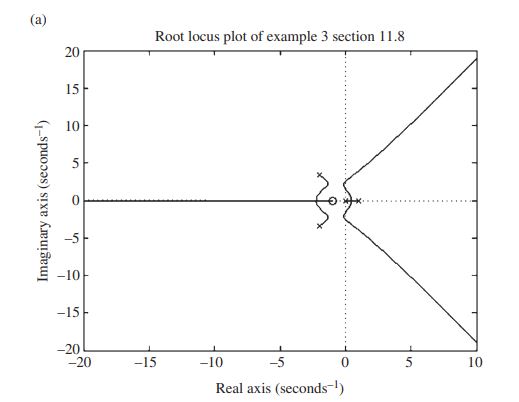
G(s)H(s)=K G_{o}(s)=\frac{K(s+1)}{s(s-1)(s^{2}+4s+16)}.
Learn more on how do we answer questions.
A simple expansion and simplification gives
G_{o}(s)=\frac{s+1}{s^{4}+3s^{2}+12s^{2}-16s}.
Therefore, the input to and output from MATLAB are included in Program Listing 11.3a and Figure 11E3a.
Note that in Figure 11E3a the loci on the right-hand side of the figure have two small parts on the left-hand half of the complex plane, meaning the system with the gains of these small parts are stable. In order to provide a better view of these two small parts, a statement is added to Program Listing 11.3a. The new program is presented as Program Listing 11.3b and the output is included in Figure 11E3b
Learn more on how do we answer questions.
Script File
Program Listing 11.3a
>> num = [0 0 0 1 1];
>> den = [1 3 12 −16 0];
>> rlocus(num,den,‘k’)
>> title(‘Root Locus Plot of Example 3 Section 11.8’)
Program Listing 11.3b
>> num = [0 0 0 1 1];
>> den = [1 3 12 -16 0];
>> rlocus(num,den,‘k’)
>> axis([−5 5 −10 10]);
>> title(‘Root Locus Plot of Example 3 Section 11.8’)