Question 19.3.a: DRIVING DISTANCES FOR GOLF BALL BRANDS If you are a golfer, ......

This example represents a controlled experiment. The consumer testing service decides exactly how to run the experiment, namely, by assigning 20 randomly chosen balls of each brand to each of three temperature levels. In our general terminology, the experimental units are the individual golf balls and the dependent variable is the length (in yards) of each drive. There are two factors: brand and temperature. The brand factor has five treatment levels, A through E, and temperature has three levels, cool, mild, and warm. The design is balanced because the same number of balls, 20, is used at each of the 5 × 3 = 15 treatment level combinations. In fact, balanced designs are the only two-way designs we will discuss in this book. (The analysis of unbalanced designs is more complex and is best left to a more advanced book.) There is one further piece of terminology. We call this a full factorial two-way design because we test golf balls at each of the 15 possible treatment level combinations. If, for example, we decided not to test any brand A balls at a temperature of 65 degrees, then the resulting experiment would be called an incomplete design. We will discuss incomplete designs briefly in the next section—and why they are sometimes used—but full factorial designs are preferred whenever possible.

In a full factorial design, we assign experimental units to each treatment level combination. In an incomplete design, we assign experimental units to some of the treatment level combinations but not to all of them.

How should the consumer testing service actually carry out the experiment? One possibility is to have 15 golfers, each of approximately the same skill level, hit 20 balls each. Golfer 1 could hit 20 brand A balls in cool weather, golfer 2 could hit 20 brand B balls in cool weather, and so on. You can probably see the downside of this design. Brand A might come out the longest ball just because the golfers assigned to brand A have good days. Therefore, if the consumer testing company decides to use human golfers, it should spread them evenly among brands and weather conditions. For example, it could employ 10 golfers to hit two balls of each brand in each of the weather conditions. Even here, however, the use of different golfers introduces an unwanted source of variation: the different abilities of the golfers (or how well they happen to be driving that day). Is the solution, then, to use a single golfer for all 300 balls? This has its own downside—namely, that the golfer might get tired in the process of hitting this many balls. Even if he hits the brands in random order, the fatigue factor could play a role in the results.

These are the types of things designers of experiments must consider. They must attempt to eliminate as many unwanted sources of variation as possible, so that any differences across the factor levels of interest can be attributed to these factors and not to extraneous factors. In this example, we suspect that the best option for the consumer testing service is to employ a “mechanical” golf ball driving machine to hit all 300 balls. This should reduce the inevitable random variation that would occur by using human golfers. Still, there will be some random variation. Even a mechanical device, hitting the same brand under the same weather conditions, will not hit every drive exactly the same length.

Once the details of the experiment have been decided and the golf balls have been hit, we will have 300 observations (yardages) at various conditions. The usual way to enter the data in Excel^\text{®}—and the only way the StatTools Two-Way ANOVA procedure will accept it—is in the stacked form shown in Figure 19.18. (See the file Golf Ball.xlsx.) There must be two categorical variables that represent the levels of the two factors (Brand and Temperature) and a measurement variable that represents the dependent variable (Yards). Although many rows are hidden in this figure, there are actually 300 rows of data, 20 for each of the 15 combinations of Brand and Temperature. Again, this is a balanced design, which is what StatTools expects for its two-way ANOVA procedure. (StatTools will issue an error message if it finds an unbalanced design, that is, unequal numbers of observations at the various treatment level combinations.)

Now that we have the data, what can we learn from them? In fact, which questions should we ask? Here it helps to look at a table of sample means, such as in Figure 19.19. (This table is part of the output from the StatTools Two-Way ANOVA procedure. Alternatively, it can be obtained easily with an Excel pivot table, as we did here.^4) Prompted by this table, here are some questions we might ask.

■ Looking at column E, do any brands average significantly more yards than any others (where these averages are averages over all temperatures)?

■ Looking at row 10, do average yardages differ significantly across temperatures (where these averages are across all brands)?

■ Looking at the columns in the range B5:D9, do differences among averages of brands depend on temperature? For example, does one brand dominate in cool weather and another in warm weather?

■ Looking at the rows in the range B5:D9, do differences among averages of temperatures depend on brand? For example, are some brands very sensitive to changes in temperature, while others are not?

It is useful to characterize the type of information these questions are seeking. Question 1 is asking about the main effect of the brand factor. If we ignore the temperature (by averaging over the various levels of it), do some brands tend to go farther than some others? This is obviously a key question for the study. Question 2 is also asking about a main effect, the main effect of the temperature factor. If we ignore the brand (by averaging over all brands), do balls tend to go farther in some temperatures than others? The answer to this question is obvious to golfers. They all know that balls compress better, and hence go farther, in warm temperatures than in cool temperatures. Therefore, this is not a key question for the study, although we would certainly expect the study to confirm what experience tells us.

Main effects indicate whether there are different means for treatment levels of one factor when averaged over the levels of the other factor.

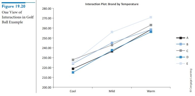
Questions 3 and 4 are asking about interactions between the two factors. These interactions are often the most interesting results of a two-way study. Essentially, interactions (if there are any) provide information that could not be guessed by knowing the main effects alone. In this example, interactions are patterns of the averages in the range B5:D9 that could not be guessed by looking only at the “main effect” averages in column E and row 10. Specifically, the order of brands in column E, from largest to smallest average yardages, is E, C, B, A, D. If there were no interactions at all, this ordering would hold at each temperature. For these data, it is close. At the cool temperature, the ordering is C, E, B, A, D; for mild, it is E, B, C, D, A; for warm, it is E, C, A, B, D. Actually, having no interactions implies even more than the preservation of these rankings. It implies that the difference between any two brands’ averages is the same at any of the three temperature levels. For example, the differences between brands E and D at the three temperatures are 224.8 − 215.0 = 9.8, 255.7 − 237.6 = 18.1, and 270.9 − 256.1 = 14.8. If there were no interactions at all, these three differences would be equal.

Interactions indicate patterns of differences in means that could not be guessed from the main effects alone. They exist when the effect of one factor on the dependent variable depends on the level of the other factor.

The concept of interaction is much easier to understand by looking at graphs. The graphs in Figures 19.20 and 19.21, which are both outputs from the StatTools Two-Way ANOVA procedure, represent two ways of looking at the pattern of averages for different combinations of brand and temperature—that is, the averages in the range B5:D9 of Figure 19.19. The first of these shows a line for each brand, where each point on the line corresponds to a different temperature. The second shows the same information with the roles of brand and temperature reversed. Neither graph is “better” than the other; they simply show the same data from different perspectives. The key to either is whether the lines are parallel. If they are, then there are no interactions—the effect of one factor on average yardage is the same regardless of the level of the other factor. The more nonparallel they are, however, the stronger the interactions are. The lines in either of these graphs are not exactly parallel, but they are nearly so. This implies that there is very little interaction between brand and temperature in these data.

In general, interactions can be of several types. We show two contrasting types in Figures 19.22 and 19.23. (For simplification, these focus on two brands only. They are based on different data from those used in the Golf Ball.xlsx file.) In Figure 19.22, brand A dominates at all temperatures. However, there is an interaction because the difference between brands increases as temperature increases. In this situation the interaction effect is interesting, but the main effect of brand—brand A is better when averaged over all temperatures—is also interesting. The situation is quite different in Figure 19.23, where there is a “crossover.” Brand A is somewhat better at cool temperatures, but brand B is better at mild and warm temperatures. In this case the interaction is the most interesting finding, and the main effect of brand is much less interesting. In simple terms, if you are a golfer, you would buy brand A in cool temperatures and brand B otherwise, and you wouldn’t care very much which brand is better when averaged over all temperatures.

For these reasons, we check first for interactions in a two-way design. If there are significant interactions, then the main effects might not be as interesting. However, if there are no significant interactions, then main effects generally become more important.

Summing up what we have seen so far, main effects are differences in averages across the levels on one factor, where these averages are averages over all levels of the other factor. In a table of sample means, such as in Figure 19.19, we can check for main effects by looking at the averages in the “Grand Total” column and row. In contrast, the interactions are patterns of averages in the main body of the table and are best shown graphically, as in Figures 19.20 and 19.21. They indicate whether the effect of one factor depends on the level of the other factor.

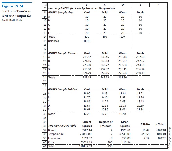
The next question is whether the main effects and interactions we see in a table of sample means are statistically significant. As in one-way ANOVA, this is answered by an ANOVA table. However, instead of having just two sources of variation, within and between, as in one-way ANOVA, there are now four sources of variation: one for the main effect of each factor, one for interactions, and one for variation within treatment level combinations. For the golf ball data, two-way ANOVA separates the total variation across all 300 observations into four sources. First, there is variation due to different brands producing different average yardages. Second, there is variation due to different average yardages at different temperatures. Third, there is variation due to the interactions we saw in the interaction graphs. Finally, there is the same type of “within” variation as in one-way ANOVA. This is the variation that occurs because yardages for the 20 balls of the same brand hit at the same temperature are not all identical. (This within variation is usually called the “error” variation in statistical software packages.)

Two-way ANOVA collects this information about the different sources of variation, using fairly complex formulas, in an ANOVA table as shown in Figure 19.24. [This is the output from StatTools, by selecting Two-Way ANOVA from the Statistical Inference group in StatTools, selecting Brand and Temperature as the categorical (C1 and C2) variables and Yards as the measurement (Val) variable. The output includes tables of sample sizes, sample means, and sample standard deviations, as well as the ANOVA table.] The four sources of variation appear in rows 37–40. Rows 37 and 38 are for the main effects of brand and temperature, row 39 is for interactions, and row 40 is for the within (error) variation. Each source has a sum of squares and a degrees of freedom. Also, each has a mean square, the ratio of the sum of squares to the degrees of freedom. Finally, the first three sources have an F-ratio and an associated p-value, where each F-ratio is the ratio of the mean square in that row to the mean square error in cell D40.

We test whether main effects or interactions are statistically significant in the usual way—by examining p-values. Specifically, we claim statistical significance if the corresponding p-value is sufficiently small, less than 0.05, say. Looking first at the interactions, the p-value is about 0.03, which says that the lines in the interaction graphs are significantly nonparallel, at least at the 5% significance level. We might dispute whether this nonparallelism is practically significant, but there is statistical evidence that at least some interaction between brand and temperature exists. The two p-values for the main effects in cells F37 and F38 are practically 0, meaning that there are differences across brands and across temperatures. Of course, the main effect of temperature was a foregone conclusion—we already knew that balls do not go as far in cold temperatures—but the main effect of brand is more interesting. According to the evidence, some brands definitely go farther, on average, than some of the others.

^4Note that the default label Excel uses in cells L10 and P4 is Grand Total—and you cannot change them. However, they are really “grand averages.”