Question 2.8: Evaluate the inductance of a strip inductor of length l = 0.......
Evaluate the inductance of a strip inductor of length l = 0.5 mm, W = 50 μm and t = 5 μm, on a 300 μm GaAs substrate (\epsilon _r=13). Assume a metal conductivity of \sigma = 4 \cdot 10^7 S/m, and tan δ = 0.001 for the GaAs substrate. Compare the input impedance of the strip inductor with the input impedance of a microstrip line having the same dimensions as a function of frequency, and find the resonant frequency of the inductor from the transmission line model. Evaluate from the lumped and distributed model the frequency behavior of inductor quality factor.
Learn more on how do we answer questions.
For the strip inductor we have L_{\text{strip}} = L_0K_{\text{g}}, where from (2.51) and (2.52)
L_{\text {strip }} =2 \cdot 10^{-1} l\left[\log \frac{l}{W+t}+1.193+\frac{W}{3 l}\right] K_\text{g}\; \text{nH}\hspace{30 pt} \text{(2.51)}\begin{aligned} K_{\text{g}} & =\left\{\begin{array}{c} 0.57-0.145 \log (W / h), \quad W / h>0.05 \\ 1, \quad W / h \leq 0.05 \end{array}\right. \end{aligned}\hspace{30 pt} \text{(2.52)}
we obtain:
\begin{aligned} L_0 & =2 \cdot 10^{-1} \times 0.5 \times\left[\log \frac{0.5}{5 \cdot 10^{-3}+50 \cdot 10^{-3}}+1.193+0.2235 \cdot \frac{50 \cdot 10^{-3}}{0.5}\right] \\ & =0.3422\> 6 \; \text{nH}, \end{aligned}
K_{\text{g}} = 0.829\> 81, L_{\text{strip}} = L_0K_{\text{g}}= 0.284\> 01 nH. The skin-effect strip resistance can be evaluated from the surface resistance
R_s=3.\> 141\> 6 \cdot 10^{-7} \sqrt{f} using (2.53):
\begin{aligned} R_{\text {strip }} & =\left[1.4+0.217 \log \left(\frac{50 \cdot 10^{-3}}{5 \times 5 \cdot 10^ {-3}}\right)\right] \frac{0.5 \times 3.\> 141\> 6 \cdot 10^{-7} \sqrt{f}}{2\left(50 \cdot 10^{-3}+5 \cdot 10^{-3}\right)} \\ & =2.\> 214\> 0 \times 10^{-6} \sqrt{f}\quad \Omega . \end{aligned}
Notice that the DC resistance of the strip is:
R_{\text {strip,DC }}=\frac{l}{W t \sigma}=\frac{0.5 \cdot 10^{-3}}{50 \cdot 10^{-6} \times 5 \cdot 10^{-6} \times 4 \cdot 10^7}=5 \cdot 10^{-2}\quad \Omega,
i.e., the skin-effect resistance at f=0.51 GHz. The input impedance finally is Z_{\text{strip}} = R_{\text{strip}}+\text{j}\omega L_{\text{strip}}. We can model the same inductor with a microstrip model, using the high-frequency expression of the characteristic parameters. Since h/W = 300/50 = 6 < 2π, we exploit the width correction (see (2.36))
\frac{W^{\prime}}{h}=\left\{\begin{aligned} \frac{W}{h}+\frac{1.25 t}{\pi h}\left[1+\log \frac{4 \pi W}{t}\right], & \quad \frac{W}{h} \leq \frac{1}{2 \pi} \\ \frac{W}{h}+\frac{1.25 t}{\pi h}\left[1+\log \frac{2 h}{t}\right], & \quad \frac{W}{h}>\frac{1}{2 \pi}. \end{aligned}\right.\hspace{30 pt} \text{(2.36)}obtaining W^{\prime}/h=0.20505 and therefore W^{\prime}=0.20505h=61.\> 515 μm; then we use the narrow strip formula (2.37)
\epsilon_{ \text{eff} }=\frac{1+\epsilon_r}{2}+\frac{\epsilon_r-1}{2} F\left(\frac{W}{h}\right)-\frac{\epsilon_r-1}{4.6} \frac{t}{h} \sqrt{\frac{h}{W}},\hspace{30 pt} \text{(2.37)}for the effective permittivity with F = 0.144 (2.38)
F\left(\frac{W}{h}\right)=\left\{\begin{array}{cl} {\left[1+\frac{12 h}{W}\right]^{-1 / 2}+0.04\left[1-\frac{W}{h}\right]^2,} &\quad \frac{W}{h} \leq 1 \\ {\left[1+\frac{12 h}{W}\right]^{-1 / 2}} &\quad \frac{W}{h}>1. \end{array}\right.\hspace{30 pt} \text{(2.38)}and \epsilon _{\text{eff}}=7.76. The impedance Z_0 and impedance in air Z_{a0} are, from (2.35),
Z_0=\left\{\begin{array}{cc} \frac{60}{\sqrt{\epsilon_{ \text{eff} }}} \log \left[\frac{8 h}{W^{\prime}}+\frac{W^{\prime}}{4 h}\right], & \frac{W^{\prime}}{h} \leq 1 \\ \frac{120 \pi}{\sqrt{\epsilon_{ \text{eff} }}}\left[\frac{W^{\prime}}{h}+1.393+0.667 \log \left(\frac{W^{\prime}}{h}+1.444\right)\right]^{-1} & \frac{W^{\prime}}{h}>1, \end{array}\right. \text{(2.35)}Z_0 = 78.9 \Omega and Z_{a0} = Z_0\sqrt{\epsilon _{\text{eff}}}=220 \Omega, respectively. This yields the total inductance lZ_{a0}/c_0 = 0.36 nH, in fair agreement with the value obtained through the concentrated model. The propagation constant is
\beta = 2πf \sqrt{\epsilon _{eff}} c_0 = 5.83 × 10^{-8}f {\text{ m}}^{-1} with the frequency in Hz. We have from (2.39) the dielectric attenuation
\alpha_d=\frac{27.3}{8.6859} \frac{13}{\sqrt{7.76}}\left(\frac{7.76-1}{13-1}\right) \frac{0.001}{3 \cdot 10^8} f=2.\> 7543 \times 10^{-11} f \text{ Np/m},
while for the conductor attenuation we use (2.34)
\lambda _c=\pi \sqrt{\epsilon _r}(a+b),\hspace{30 pt} \text{(2.34)}yielding \Lambda = 15.134 and from (2.33):
\alpha_c=\frac{9.5 \times 10^{-5}(a+b) \sqrt{\epsilon_r}}{a b \log (b / a)} \sqrt{f_{ \text{GHz} }}\text{ dB/m}.\hspace{30 pt} \text{(2.33)}\begin{aligned} \alpha_c & =\frac{1.38}{8.6859} \frac{R_s}{h Z_0} \frac{32-\left(W^{\prime} / h\right)^2}{32+\left(W^{\prime} / h\right)^2} \Lambda \\ & =\frac{1.38}{8.6859} \frac{3. 141 6 \cdot 10^{-7} \sqrt{f}}{300 \cdot 10^{-6} \cdot 78.9} \frac{32-0.20505^2}{32+0.20505^2} \times 15.\> 134 \\ & =3.\> 182\> 9 \times 10^{-5} \sqrt{f} \text{ Np/m}. \end{aligned}
The input impedance of the shorted line therefore is:
Z_{\text{line}} = Z_0 \text{ tanh }[(\alpha _c + \alpha _d + \text{j}\beta ) l].
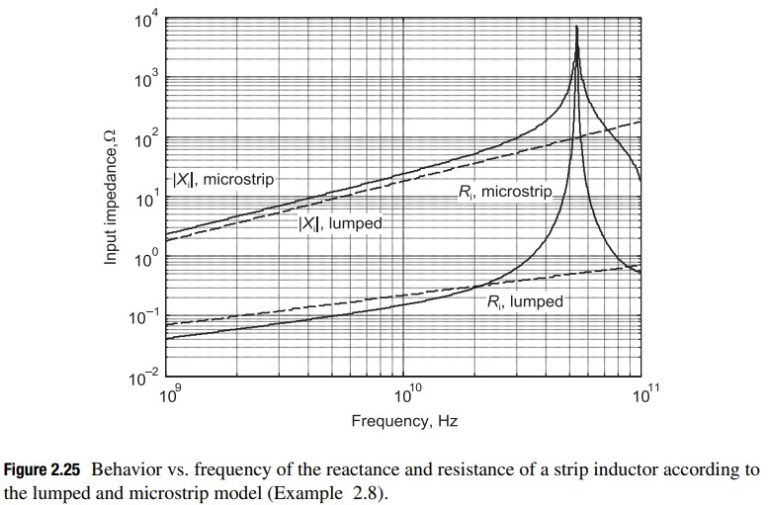
The magnitudes of the reactance and resistance evaluated from the lumped and the microstrip model are shown in Fig. 2.25; the microstrip model yields a resonance around 55 GHz. The limit l < \lambda_{\text{g}}/10 would confine the frequency range of the inductor to frequencies below 22 GHz. Concerning the quality factor, we have:
Q_L=\frac{\omega L_{\text {strip }}}{R_{\text {strip }}}=\frac{2 \pi f \times 0.284\> 01 \cdot 10^{-9}}{2.\> 214\> 0 \times 10^{-6} \sqrt{f}}=8.\> 06 \times 10^{-4} \sqrt{f},
while from the microstrip model Q_L = {\text{Im }} [Z_{\text{line}}] /\text{Re } [Z_{\text{line}}]. The behavior of the quality factor evaluated from the lumped and the microstrip model is shown in Fig. 2.26; while according to the lumped model the quality factor increases monotonically, in the microstrip model this has a maximum and then drops owing to the element resonance.