Question 11.SP.7: For the uniform beam and loading shown, determine the reacti......
For the uniform beam and loading shown, determine the reactions at the supports.
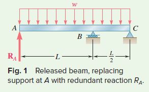
STRATEGY: The beam is indeterminate to the first degree, and we must choose one of the reactions as a redundant. We then use a free-body diagram to solve for the reactions due to the distributed load and the redundant reaction. Using free-body diagrams of the segments, we obtain the moments as a function of the coordinate along the beam. Using Eq. (11.57), we write Castigliano’s theorem for deflection associated with the redundant reaction. We set this deflection equal to zero, and solve for the redundant reaction. Equilibrium can then be used to find the other reactions.
x_j=\frac{\partial U}{\partial P_j}=\int_0^L \frac{M}{E I} \frac{\partial M}{\partial P_j} d x (11.57)

Learn more on how do we answer questions.
MODELING and ANALYSIS:
Castigliano’s Theorem. Choose the reaction R _A as the redundant one (Fig. 1). Using Castigliano’s theorem, determine the deflection at A due to the combined action of R _A and the distributed load. Since EI is constant,
y_A=\int \frac{M}{E I}\left(\frac{\partial M}{\partial R_A}\right) d x=\frac{1}{E I} \int M \frac{\partial M}{\partial R_A} d x (1)
The integration will be performed separately for portions AB and BC of the beam. R _A is then obtained by setting y _A equal to zero.
Free Body: Entire Beam. Using Fig. 2, the reactions at B and C in terms of R _A and the distributed load are
R_B=\frac{9}{4} w L-3 R_A \quad R_C=2 R_A-\frac{3}{4} w L (2)
Portion AB of Beam. Using the free-body diagram shown in Fig. 3, find
M_1=R_A x-\frac{w x^2}{2} \quad \frac{\partial M_1}{\partial R_A}=x
Substituting into Eq. (1) and integrating from A to B gives
\frac{1}{E I} \int M_1 \frac{\partial M}{\partial R_A} d x=\frac{1}{E I} \int_0^L\left(R_A x^2-\frac{w x^3}{2}\right) d x=\frac{1}{E I}\left(\frac{R_A L^3}{3}-\frac{w L^4}{8}\right) (3)
Portion BC of Beam. Using the free-body diagram shown in Fig. 4, find
M_2=\left(2 R_A-\frac{3}{4} w L\right) ν-\frac{w ν^2}{2} \quad \frac{\partial M_2}{\partial R_A}=2 ν
Substituting into Eq. (1) and integrating from C (where ν = 0) to B (where ν=\frac{1}{2} L ) gives
\frac{1}{E I} \int M_2 \frac{\partial M_2}{\partial R_A} d ν=\frac{1}{E I} \int_0^{L / 2}\left(4 R_A ν^2-\frac{3}{2} w L ν^2-w ν^3\right) d ν
=\frac{1}{E I}\left(\frac{R_A L^3}{6}-\frac{w L^4}{16}-\frac{w L^4}{64}\right)=\frac{1}{E I}\left(\frac{R_A L^3}{6}-\frac{5 w L^4}{64}\right) (4)
Reaction at A. Adding the expressions from Eqs. (3) and (4), we obtain y_A and set it equal to zero:
y_A=\frac{1}{E I}\left(\frac{R_A L^3}{3}-\frac{w L^4}{8}\right)+\frac{1}{E I}\left(\frac{R_A L^3}{6}-\frac{5 w L^4}{64}\right)=0
Thus, R_A=\frac{13}{32} w L \quad R _A=\frac{13}{32} w L \uparrow
Reactions at B and C. Substituting for R_A into Eq. (2), we obtain
R _B=\frac{33}{32} w L \uparrow \quad R _C=\frac{w L}{16} \uparrow