Question 19.2: PAYMENTS FOR ORDERS AT REBCO Rebco is a manufacturing compan......
PAYMENTS FOR ORDERS AT REBCO
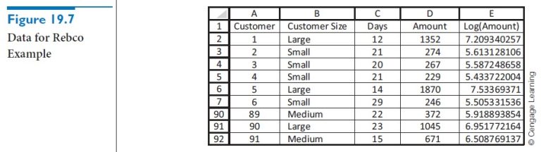
Rebco is a manufacturing company that supplies parts to many other manufacturing companies, its customers. Rebco is concerned about the time it takes these customers to pay for their orders. The file Rebco Payments.xlsx contains data (a subset of which is shown in Figure 19.7) on the most recent payment from 91 of its customers. The customers are categorized as small, medium, and large. For each customer we see the number of days it took the customer to pay and the amount of the payment. Are there any differences in the mean time to pay across the three customer sizes? What about differences across the mean payment amounts?
Objective To see how a logarithm transformation can be used to ensure the validity of the ANOVA assumptions, and to see how the resulting output should be interpreted.
Learn more on how do we answer questions.
Unlike Example 19.1, this is a one-factor observational study, where the single factor is customer size at three levels: small, medium, and large. The experimental units are the bills for the orders, and there are two dependent variables, days until payment and payment amount, that will be examined. Focusing first on the days until payment, you can see from the side-by-side box plots in Figure 19.8 that whatever differences there are appear to be slight. Perhaps the large customers pay, on average, a bit more promptly, but it is difficult to see from the plots whether the apparent differences are significant. Therefore, we turn to the numerical results. The summary results and the ANOVA table in Figure 19.9 show that the differences between the sample means are not even close to being statistically significant. The p-value for the test is only 0.318. Rebco cannot reject the null hypothesis that customers of all sizes take, on average, the same number of days to pay.
The analysis of the amounts these customers pay is quite different. This is immediately evident from the side-by-side box plots in Figure 19.10. Actually, two things are clear. First, there is little doubt that small customers tend to have lower bills than medium-size customers, who in turn tend to have lower bills than large customers. Second, however, you can see that the equal-variance assumption is grossly violated. There is very little variation in payment amounts from small customers and a large amount of variation from large customers. This situation should be remedied before running any formal ANOVA.
One common method for equalizing variances is to take logarithms of the dependent variable and then use the transformed variable as the new dependent variable. This log transformation tends to spread apart small values and compress together large values— exactly what is needed in this example. After taking the logarithms of the payment amounts, we obtain the box plots in Figure 19.11. The log transformation retains the ordering, so that logs of small amounts are still less than logs of large amounts, but the variances are now much closer to being equal. The resulting ANOVA on the log variable appears in Figure 19.12. The p-value in the ANOVA table is again the key for checking whether we can reject the equal-means hypothesis. The fact that it is virtually 0 indicates that the means of the log variables are not equal.
What does this say about the original variables? The bottom part of the output in Figure 19.12 answers this question, although we have to be very careful when interpreting the results. First, when we ran the StatTools One-Way ANOVA procedure on the log of the Amount variable, we requested the confidence intervals in rows 32–34.² However, each of these is a confidence interval for the difference between means of the log-transformed variables. Because they are in log units, these numbers have little practical meaning. The trick is to take their antilogarithms (with the EXP function), as shown in rows 37–39, and then interpret the antilogs correctly. It can be shown that the correct interpretation is that each antilog is a ratio of medians for the respective treatment levels. (If the populations are reasonably symmetric, the antilogs can also be interpreted as approximate ratios of means.) For example, our best guess is that the median amount paid by large customers is 2.253 times as large as the median amount paid by medium-sized customers, and we are 95% confident that this ratio is between 1.877 and 2.705. Because the populations are reasonably symmetric (see the box plots in Figure 19.10), this same statement applies, at least approximately, to the means.
The bottom line for Rebco is that its large customers have bills that are typically over twice as large as those for medium-sized customers, which in turn are typically over twice as large as those for small customers. Even though all customers currently tend to take about the same number of days to pay, there is a greater incentive to get the large customers to pay early—more money is at stake.
²Again, we will discuss the type of confidence interval method shown here in Section 19-4.


