Question 6.AE.9: The drive motor of a piston compressor is a nonsalient-pole ......

a) n_{\mathrm{ms}}=(120 \cdot \mathrm{f}) / p=257.14 \mathrm{rpm}, \omega_{\mathrm{ms}}=\left(2 \pi \cdot n_{\mathrm{ms}}\right) / 60=26.927 \mathrm{rad} / \mathrm{s}.

T_{\mathrm{rat}}=\frac{P_{\mathrm{rat}}}{\omega_{m \mathrm{~s}}}=278.53 \mathrm{kNm}        (E6.9-5)

\left|\tilde{I}_{a_{-} \mathrm{rat}}\right|=\frac{\mathrm{P}_{\mathrm{rat}}}{\sqrt{3} \cdot V_{L-L \mathrm{rat}} \cos \varphi_{\mathrm{rat}} \eta_{\mathrm{rat}}}=827.6 \mathrm{~A}            (E6.9-6)

The average load torque T_{Lavg}=265.53 kNm leads with

T_{L avg}=\frac{3\left|\widetilde{E}_a\right|\left|\widetilde{V}_{a \_ \text {rat }}\right|}{X_s \omega_{m s}} \sin \delta \text { and } T_{\max }=\frac{3\left|\widetilde{E}_a\right|\left|\widetilde{V}_{a \_ \text {rat }}\right|}{X_s \omega_{m s}}

to the ratio

\begin{aligned} \frac{T_{\text {Lavg }}}{T_{\max }} & =\sin \delta \text { or } \delta=\sin ^{-1}\left(\frac{T_{\text {Lavg }}}{2.3 \cdot T_{\text {rat }}}\right) \\ & =0.427 \mathrm{rad} \text { or } 24.48^{\circ} . \end{aligned}              (E6.9-7)

Figure E6.9.1 defines the torque angle δ.
From the phasor diagram (overexcited, consumer notation) one obtains

\left|\widetilde{E}_a\right|^2=\left(\left|\widetilde{V}_{a \_\mathrm{rat}}\right|+\left|\widetilde{I}_a\right| X_s \sin \varphi\right)^2+\left(\left|\widetilde{I}_a\right| X_s \cos \varphi\right)^2

or

\left|\widetilde{E}_a\right|^2=\left|\tilde{V}_{a\_rat }\right|^2+2\left|\tilde{V}_{a\_rat }\right|\left|\tilde{I}_a\right| X_s \sin \varphi+\left(\left|\tilde{I}_a\right| X_s\right)^2  (E6.9-8)

and with

P=\frac{3\left|\widetilde{E}_a\right|\left|\widetilde{V}_{a\_rat }\right| \sin \delta}{X_s}              (E6.9-9)

follows the second-order equation for X_S.

\begin{aligned} & {\left[\left(\frac{P}{3\left|\tilde{V}_{a_{-} \mathrm{rat}}\right| \sin \delta}\right)^2-\left|\widetilde{I}_a\right|^2\right] X_s^2} \\ & -\left(2\left|\widetilde{V}_{a_{\_} \mathrm{rat}}\right|\left|\widetilde{I}_a\right| \sin \varphi\right) X_s-\left|\widetilde{V}_{a_{-} \mathrm{rat}}\right|^2=0 . \end{aligned}            (E6.9-10)

For the given operating point one gets

P=T_{\text {Lavg }} \cdot \omega_{m s}=7.14 \mathrm{MW},\left|\widetilde{V}_{a_{-} \mathrm{rat}}\right|=3.464 \mathrm{kV},

\begin{aligned} & \sin \delta=\frac{T_{\mathrm{Lavg}}}{T_{\max }}=\frac{T_{\mathrm{Lavg}}}{2.3 \cdot T_{\mathrm{rat}}}=0.4145 \\ & \cos \varphi=0.9, \sin \varphi=0.4359 \end{aligned}              (E6.9-11)

cosφ = 0:9, sinφ = 0:4359,

\left|\widetilde{I}_a\right|=\frac{T_{\text {Lavg }} \cdot \omega_{m s}}{3 \cdot\left|\widetilde{V}_{a_{-} \mathrm{rat}}\right| \cdot \cos \varphi \cdot \eta_{\mathrm{rat}}}=789 \mathrm{~A}

and therefore

X_s = 3:07 Ω.                            (E6.9-12)

With the base impedance of

Z_{\text {base }}=\frac{\left|\tilde{V}_{a \_ \text {rat }}\right|}{\left|\widetilde{I}_{a \_ \text {rat }}\right|}=4.18 \Omega              (E6.9-13)

the per-unit synchronous reactance is

X_{s\_pu} = 0:74 pu              (E6.9-14)

b) Nonlinear differential equation for the motor torque.
The torque equation is

T-T_L-J \frac{d \omega_m}{d t}=0              (E6.9-15

where

\begin{aligned} T & =T_{\max } \cdot \sin \delta, \delta=\frac{p}{2} \alpha, T_L=T_{L a vg}+T_{L 1}, \\ \alpha & =\omega_{m s} t-\omega_m t, \frac{d \alpha}{d t}=\left(\omega_{m s}-\omega_m\right), \frac{d \delta}{d t}=\frac{p}{2} \cdot \frac{d \alpha}{d t}, \\ \frac{d \delta}{d t} & =\frac{p}{2}\left(\omega_{m s}-\omega_m\right), \omega_m=\omega_{m s}-\frac{1}{p / 2} \cdot \frac{d \delta}{d t}, \\ \frac{d \omega_m}{d t} & =-\frac{1}{p / 2} \frac{d^2 \delta}{d t^2}\quad (E6.9-16) \end{aligned}

The nonlinear differential equation becomes

T_{\max } \sin \delta-T_{L a v g}-T_{L 1}+\frac{J}{p / 2} \frac{d^2 \delta}{d t^2}=0              (E6.9-17)

Linearization of the nonlinear differential equation is based on Fig. E6.9.2.

The motor torque is

T=T_{\max } \sin \left(\delta_0+\delta_1\right)=T_{\max } \sin \delta_0+T_{\max } \delta_1 \cos \delta_0            (E6.9-18)
or with the synchronizing torque S=T_{max} cos δ_o, the linearized differential equation becomes

\delta_1+\frac{J}{(p / 2) S} \frac{d^2 \delta_1}{d t^2}=\frac{T_{L 1}}{S}              (E6.9-19)

The eigen-angular frequency of the undamped machine can be defined by

\omega_{\text {eigen }}=\sqrt{\frac{(p / 2) S}{J}}            (E6.9-20)

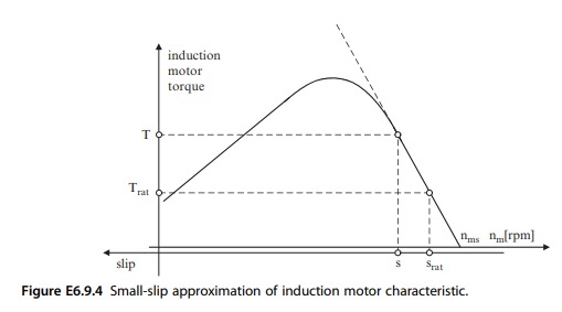
c) Repetition of part b, but not neglecting damping provided by induction motor action as is indicated in Fig. E6.9.3. The small-slip approximation of an induction motor is depicted in Fig. E6.9.4.
From Fig. E6.9.4 one obtains for the motor torque developed by induction-motor action

\begin{aligned} & T_{\text {induction }}=\frac{T_{\mathrm{rat}} \cdot s}{s_{\mathrm{rat}}}, s=1-\frac{n_m}{n_{m s}}=1-\frac{\omega_m}{\omega_{m s}}, \\ & T_{\text {induction }}=\frac{T_{\mathrm{rat}}}{s_{\mathrm{rat}}}\left(1-\frac{\omega_m}{\omega_{m \mathrm{~s}}}\right),\quad (E6.9-21a \end{aligned}

or

T_{\text {induction }}=\frac{T_{\text {rat }}}{s_{\mathrm{rat}}} \frac{1}{(p / 2) \cdot \omega_{m s}} \cdot \frac{d \delta}{d t} .                  (E6.9-21b)

With the power system’s frequency ω_s=2πf and ω_s=(p/2)ω_{ms} one obtains the total motor torque

T=T_{\max } \sin \delta+\frac{T_{\mathrm{rat}}}{s_{\mathrm{rat}}} \cdot \frac{1}{\omega_s} \cdot \frac{d \delta}{d t}            (E6.9-21c)

or the nonlinear differential equation including the damping due to induction-motor action

\frac{J}{(p / 2)} \frac{d^2 \delta}{d t^2}+\frac{T_{\mathrm{rat}}}{s_{\mathrm{rat}} \cdot \omega_s} \frac{d \delta}{d t}+T_{\max } \sin \delta=T_{L avg}+T_{L 1}                      (E6.9-22)

Linearization leads to the differential equation

\frac{J}{(p / 2)} \frac{d^2 \delta_1}{d t^2}+D \frac{d \delta_1}{d t}+S \delta_1=T_{L 1},(\mathrm{E} 6.9-23)

where the damping factor is

D=\frac{T_{\mathrm{rat}}}{s_{\mathrm{rat}} \cdot \omega_s}            (E6.9-24)

d) Solution of the linearized differential equations of part b – without damping – and determining (by introducing phasors indicated by “˜”) the axial moment of inertia J required so that the first harmonic motor torque T_1(t) will be reduced to ± 4% of the average torque (Eq. E6.9-2).
Neglecting damping one obtains for the kth harmonic the differential equation

\delta_1+\frac{1}{\omega_{\text {eigen }}^2} \frac{d^2 \delta_1}{d t^2}=\frac{T_{L k}}{S} .                (E6.9-25)

Replacing \frac{d}{d t} \text { by } j \omega_k for sine/cosine variations of harmonic torques one gets

\widetilde{\delta}_1+\frac{1}{\omega_{\text {eigen }}^2}\left(j \omega_k\right)^2 \widetilde{\delta}_1^2=\frac{\widetilde{T}_{L k}}{S}              (E6.9-26)

With

\widetilde{T}_k=T_{\max } \cos \tilde{\delta}_0 \widetilde{\delta}_1=S \cdot \widetilde{\delta}_1            (E6.9-27)

follows

\frac{\widetilde{T}_k}{\widetilde{T}_{L k}}=\frac{1}{\left(1-\frac{\omega_k^2}{\omega_{\text {eigen }}^2}\right)}            (E6.9-28)

or magnitudes only where “^” indicates amplitude

\frac{\left|\widetilde{T}_k\right|}{\left|\widetilde{T}_{L k}\right|} \equiv \frac{\hat{T}_k}{\hat{T}_{L k}}=\frac{1}{\left[1-\left(\frac{\omega_k}{\omega_{\text {eigen }}}\right)^2\right]}            (E6.9-29)

where \tan (\varepsilon)=0 \text { for } \omega_k<\omega_{\text {eigen }} \text { and } \tan (\varepsilon)=-180^{\circ} \text { for } \omega_{\mathrm{k}}>\omega_{\text {eigen }} (see E6.9-38).
For the first harmonic torque one can write

T_{L 1}=31.04 \mathrm{kNm} \sin \left(\omega_{m s} t-\pi\right), \hat{T}_1=\pm 0.04 T_{L a v g}              (E6.9-30)

\frac{\hat{T}_1}{\hat{T}_{L 1}}=\frac{1}{\left(1-\frac{\omega_1^2}{\omega_{\text {eigen }}^2}\right)}              (E6.9-31)

The required inertia becomes for the worst case (– sign):

\begin{aligned} J=\frac{S(p / 2)}{\omega_1^2}\left(1-\frac{\hat{T}_{L 1}}{\hat{T}_1}\right) & =\frac{2.3 \cdot T_{\mathrm{rat}} \cdot \cos \delta_o \cdot(p / 2)^3}{\omega_s^2} \\ \left(1-\frac{\hat{T}_{L 1}}{\hat{T}_1}\right) & =11.256 \cdot 10^3\left(1-\frac{31.04}{\pm 0.04 \cdot 265.53}\right) \\ & =44 \cdot 10^3 \mathrm{kgm}^2 \end{aligned}                    (E6.9-32)

Solution of the linearized differential equations of part c – with damping – and determining (by introducing phasors) the axial moment of inertia J required so that the first harmonic motor torque will be reduced to Not neglecting damping one obtains for the kth har ± 4% of the average torque (Eq. E6.9-2).
Not neglecting damping one obtains for the kth harmonic the differential equation

\frac{J}{(p / 2)} \frac{d^2 \delta_1}{d t^2}+D \frac{d \delta_1}{d t}+S \delta_1=T_{L k}          (E6.9-33)

or for sine/cosine variations of harmonic load torques

\left(j \omega_k\right)^2 \frac{J}{(p / 2)} \cdot \widetilde{\delta}_1+j \omega_k D \widetilde{\delta}_1+S \widetilde{\delta}_1=\widetilde{T}_{L k}            (E6.9-34)

with

\widetilde{S \delta}_1=\widetilde{T}_k              (E6.9-35)

\frac{\widetilde{T}_k}{\widetilde{T}_{L k}}=\frac{1}{\left(j \omega_k\right)^2 \cdot \frac{J}{(p / 2) \cdot S}+j \omega_k \frac{D}{S}+1}                  (E6.9-36)

or the magnitudes only

\frac{\left|\widetilde{T}_k\right|}{\left|\widetilde{T}_{L k}\right|} \equiv \frac{\hat{T}_k}{\hat{T}_{L k}}=\frac{1}{\sqrt{\left(1-\omega_k^2 \frac{J}{(p / 2) \cdot S}\right)^2+\left(\omega_k \frac{D}{S}\right)^2}}            (E6.9-37)

with

\tan (\varepsilon)=\frac{\omega_k \frac{D}{S}}{1-\omega_k^2 \frac{J}{(p / 2) \cdot S}}              (E6.9-38)

The inertia is now

J=\frac{(p / 2) \cdot S}{\omega_k^2}\left[1 \mp \sqrt{\left(\frac{\hat{T}_{L k}}{\hat{T}_k}\right)^2-\left(\omega_k \cdot \frac{D}{S}\right)^2}\right]              (E6.9-39)

With

\begin{aligned} & \omega_k=\omega_{m s}=\frac{\omega_s}{(p / 2)}, \hat{T}_{L k}=\hat{T}_{L 1}=31.04 \mathrm{kNm} \\ & \hat{T}_k=\hat{T}_1=0.04 \cdot 265.53 \mathrm{kNm}=10.62 \mathrm{kNm} \end{aligned}

one obtains with D and S defined above

J=43.66 \cdot 10^3 \mathrm{kgm}^2 \approx 44 \cdot 10^3 \mathrm{kgm}^2            (E6.9-40)

Conclusion. Damping does not significantly influence the calculation of the required axial moment of inertia
e) Comparison of the eigen frequency f_{eigen} with the pulsation frequencies occurring at the eccentric shaft.
The angular eigen (resonance) frequency of the undamped oscillation is

\omega_{\text {eigen }}=\sqrt{\frac{S(p / 2)}{J}}=13.62 \mathrm{rad} / \mathrm{s}

or the eigen frequency is

f_{\text {eigen }}=\frac{\omega_{\text {cigen }}}{2 \pi}=2.17 \frac{1}{\mathrm{~s}} \text {. }

The first harmonic pulsation (given by the load) frequency of the eccentric shaft is

\omega_1=\omega_{m s}=\frac{\omega_s}{(p / 2)}=\frac{2 \pi 60}{14}=26.93 \frac{1}{s}              (E6.9-41)

The ratio between first harmonic pulsation frequency and resonance frequency is

\frac{\omega_1}{\omega_{\text {eigen }}}=\frac{f_1}{f_{\text {eigen }}}=1.98 \approx 2.0 .              (E6.9-42)

The fourth harmonic pulsation (given by the load) frequency of the eccentric shaft is

\omega_4=4 \cdot \omega_{m s}=4 \cdot \omega_1 .            (E6.9-43)

The ratio between fourth harmonic pulsation frequency and resonance frequency is

\frac{\omega_4}{\omega_{\text {eigen }}}=\frac{f_4}{f_{\text {eigen }}}=4 \cdot 1.98 \approx 8.0 .              (E6.9-44)

Note that from a dynamic performance point of view it is desirable if

\frac{\omega_k}{\omega_{\text {eigen }}} \geq 3-4                (E6.9-45)

As can be seen the ratio \omega_1 / \omega_{\text {eigen }}=1.98 \approx 2.0 does not satisfy this condition and therefore the calculated axial moment of inertia of 44.10³ kgm² is not large enough. It is recommended to select a desirable axial moment of inertia of J_{desirable} that is larger than 44.10³ kgm² and results in \omega_1 / \omega_{\text {eigen }} \approx 3.0.

f) List the total motor torque T(t) as a function of time (neglecting damping) for one revolution of the eccentric shaft and compare it with the load torque T_L(t). Why are they different?

The total motor torque is now

\vec{T}=\vec{T}_{\text {Lavg }}+\vec{T}_1+\vec{T}_4                (E6.9-46)

where

\vec{T}_{\text {Lavg }}=265.53 \mathrm{k} \mathrm{Nm}              (E6.9-47)

and the motor torque for the kth harmonic is

\vec{T}_k=\frac{\vec{T}_{L k}}{1-\left(\frac{\omega_k^2}{\omega_{\text {eigen }}^2}\right)}              (E6.9-48)

For the first harmonic load torque one obtains

\begin{aligned} T_{L 1}(t) & =31.04 \mathrm{kNm} \sin \left(\omega_{m s} t-\pi\right) \\ & =-31.04 \mathrm{kNm} \sin \left(\omega_{m s} t\right) \end{aligned}                  (E6.9-49)

and the first harmonic motor torque becomes

T_1(t)=\frac{-31.04 \mathrm{kNm}}{1-\left(\frac{\omega_1^2}{\omega_{\text {eigen }}^2}\right)} \sin \omega_{m s} t=10.35 \mathrm{kNm} \sin \left(\omega_{m s} t\right)          (E6.9-50)

For the fourth harmonic motor torque one gets

\begin{aligned} T_4(t) & =\frac{50.65 \mathrm{kNm}}{1-\left(\frac{\omega_4^2}{\omega_{\text {eigen }}^2}\right)} \sin \left(4 \omega_{m s} t-\frac{\pi}{6}\right) \\ & =-0.804 \mathrm{kNm} \sin \left(4 \omega_{m s} t-\frac{\pi}{6}\right) . \end{aligned}                    (E6.9-51)

Conclusions. The total load torque is

\begin{aligned} T_L(t)= & 265.53 \mathrm{kNm}+31.04 \mathrm{kNm} \sin \left(\omega_{m s} t-\pi\right) \\ & +50.65 \mathrm{kNm} \sin \left(4 \omega_{\mathrm{ms}} t-\pi / 6\right) \end{aligned}                (E6.9-52)

and the total motor torque becomes

\begin{aligned} T(t)= & 265.53 \mathrm{kNm}+10.35 \mathrm{kNm} \sin \left(\omega_{m s} t\right) \\ & -0.804 \mathrm{kNm} \sin \left(4 \omega_{m s} t-\frac{\pi}{6}\right) . \end{aligned}

The difference in the harmonic torques is provided by the flywheel with inertia of J=44.10³ kgm² .