Question 11.6: The objective of this example is to numerically verify the t......
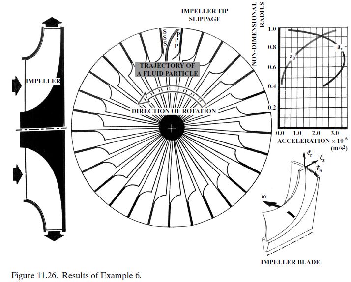
The objective of this example is to numerically verify the theoretical rationale with which the “slip-phenomenon” section was introduced. The computational procedure here is consistent with this rationale. In other words, we will calculate each of the centripetal and Coriolis acceleration components, these being the two predominant components, weighing each magnitude, as we follow a fluid particle in the blade-to-blade passage. In doing so, it is important to define a right-handed cylindrical frame of reference in order to ensure the correct signs of the different acceleration components (Fig. 11.26).
Figure 11.25 shows a centrifugal compressor stage and the major geometrical variables. These variables have the following magnitudes:
• Mean inlet radius (r_{1}) = 4.6 cm
• Exit radius (r_{2}) = 10.5 cm
• Inlet blade height (h_{1}) = 5.2 cm
• Exit blade width (b_{2}) = 1.8 cm
The stage design point gives rise to the following set of data:
• Rotational speed (N) = 41,600 rpm
• Inlet total pressure (p_{t\ 1}) = 1.88 bars
• Inlet total temperature (T_{t\ 1}) = 490 K
• Inlet swirl angle (α_{1}) = 0
• Exit total pressure (p_{t\ 2}) = 6.02 bars
• Exit total temperature (T_{t\ 2}) = 683 K
• Radial blading, with no deviation angle (i.e., β_{2} = 0)
• Slip factor (\sigma_{s}) = 92.6%
• Choked flow at the impeller inlet station (i.e., W_{1}/W_{cr\ 1} = 1.0)
• Sonic flow at the impeller outlet (i.e., V_{2}/V_{cr\ 2} = 1.0)
Assuming a parabolic dependency of the velocity components (V_{r} and V_{θ} ) on the radius (r ) (Fig. 11.25), calculate the components of both the Coriolis and centripetal accelerations at key radial locations of your choice. Use the results to explain the tangential shifting of a fluid particle which is traversing the impeller subdomain.

Learn more on how do we answer questions.
Referring to the inlet velocity diagram in Figure 11.25, we get
W_{\theta\ 1}=U_{1}=209.1\,\mathrm{m/s}
T_{t\ r\ 1}=T_{t\ 1}+{\frac{\left(W_{\theta\ 1}{}^{2}-V_{\theta\ 1}{}^{2}\right)}{2c_{p}}}=T_{t\ 1}+{\frac{W_{\theta\ 1}{}^{2}}{2c_{p}}}=496.8\,\mathrm{K}
W_{c\ r\ 1}=\sqrt{\left(\frac{2\gamma}{\gamma+1}\right)R T_{t\ r\ 1}}=407.8\,\mathrm{m/s}
W_{1}=W_{c r\ 1}=407.8\,\mathrm{m/s}
V_{1}=V_{z1}={\sqrt{W_{1}{}^{2}-U_{1}{}^{2}}}=350.2\,{\mathrm{m/s}}
V_{c r\ 1}={\sqrt{\left({\frac{2\gamma}{\gamma+1}}\right)R T_{t\ 1}}}=405.1\,{\mathrm{m/s}}
M_{c r\ 1}={\frac{V_{1}}{V_{c r\ 1}}}=0.88
\rho_{1}=\frac{p_{t\ 1}}{R T_{t\ 1}}\biggl[1-\biggl(\frac{\gamma-1}{\gamma+1}\biggr)M_{c r\ 1}{}^{2}\biggr]^{\frac{1}{\gamma-1}}=0.976\,\mathrm{kg/m}^{3}
\dot{m}=\rho_{1}V_{z1}(2\pi r_{1}h_{1})=5.14\,\mathrm{kg/s}
Referring to the exit velocity diagram in Fig. 11.25, we can calculate the following exit variables:
V_{c r\ 2}=\sqrt{\left(\frac{2\gamma}{\gamma+1}\right)R T_{t\ 2}}=478.2\,{\mathrm{m/s}}
V_{2}=V_{c r\ 2}=478.2\ {\mathrm{m/s}}
(V_{\theta\ 2})_{i d.}=U_{2}=457.4\,\mathrm{m/s}
(V_{\theta\ 2})_{a c t.}=\sigma_{s}(V_{\theta\ 2})_{i d.}=423.6\,\mathrm{m/s}
V_{r\ 2}={\sqrt{V_{2}{}^{2}-V_{\theta\ 2}{}^{2}}}=222.0\,\mathrm{m/s}
PARABOLIC INTERPOLATION OF V_{r} AND V_{θ}:
Let us define the nondimensional radial coordinate \bar{r} as follows:
{\bar{r}}={\frac{r-r_{1}}{r_{2}-r_{1}}}
Using the impeller-exit magnitudes of V_{r} and V_{θ} as boundary conditions, we get the following two parabolic relationships:
V_{r}=222.0\ \bar{r}^{2}
V_{\theta}=423.6\ \bar{r}^{2}
Referring back to Example 7 in Chapter 9, and noting that the rotational speed ω is opposite to the θ direction, we can express the combined centripetal and Coriolis acceleration components as
(a)_{n e t}=[(\omega^{2}r)-2(\omega W_{\theta})]e_{r}+[2\omega W_{r}]e_{\theta}
Noting that W_{θ} = V_{θ} − ω_{r} , we can now calculate the net acceleration components at the following five radial locations:
(a_{r})_{\bar{r}=0.2}=3.14\times10^{6}\,\mathrm{m}/\mathrm{s}^{2}\quad\mathrm{and}\quad(a_{\theta})_{\bar{r}=0.2}=0.08\times10^{6}\,\mathrm{m}/\mathrm{s}^{2}
(a_{r})_{\bar{r}=0.4}=3.38\times10^{6}\,\mathrm{m/s^{2}}\quad\mathrm{and}\quad(a_{\theta})_{\bar{r}=0.4}=0.31\times10^{6}\,\mathrm{m/s^{2}}
(a_{r})_{\bar{r}=0.6}=3.30\times10^{6}\,\mathrm{m}/\mathrm{s}^{2}\quad\mathrm{and}\quad(a_{\theta})_{\bar{r}=0.6}=0.70\times10^{6}\,\mathrm{m}/\mathrm{s}^{2}
(a_{r})_{\bar{r}=0.8}=2.95\times10^{6}\,\mathrm{m}/\mathrm{s}^{2}\quad\mathrm{and}\quad(a_{\theta})_{\bar{r}=0.8}=1.24\times10^{6}\,\mathrm{m}/\mathrm{s}^{2}
(a_{r})_{\bar{r}=1.0}=2.29\times10^{6}\,\mathrm{m}/\mathrm{s}^{2}\quad\mathrm{and}\quad(a_{\theta})_{\bar{r}=1.0}=1.94\times10^{6}\,\mathrm{m}/\mathrm{s}^{2}
A plot of these results is shown in Figure 11.26, where the following conclusions can be drawn:
• The radial-acceleration component continues to decline as the impeller exit station is approached. This is due to the decline in the Coriolis-acceleration radial component. As a result, a fluid particle in this region will continually lose radial momentum.
• Over the same exit subregion, the tangential component of Coriolis acceleration continuously grows, causing the tangential shift of a fluid particle that is sketched and labeled “particle trajectory” in Figure 11.26.
• Combination of the two flow behavioral characteristics (above) gives rise to the slip phenomenon, which was qualitatively discussed earlier in this chapter.