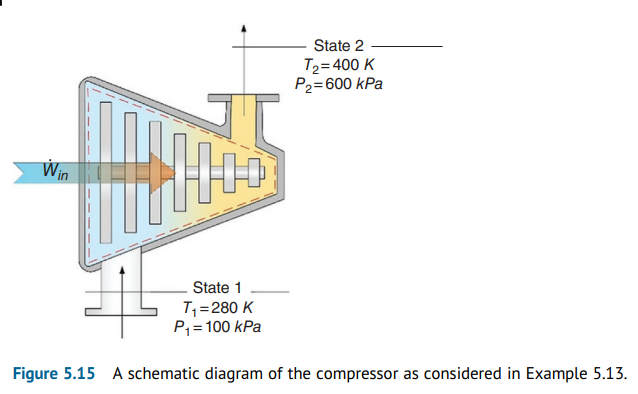
One may start with some assumptions: (i) the heat losses occur in the compression process, (ii) the changes in the kinetic and potential energies of air are negligible, and (iii) the air is treated as an ideal gas.
a) Write the mass, energy, entropy, and exergy balance equations for the air compressor.
MBE : \dot{m}_{1}=\dot{m}_{2}EBE : \dot{m}_{1} h_{1}+\dot{W}_{\text {in }}=\dot{m}_{2} h_{2}+\dot{Q}_{\text {out }}
EnBE : \dot{m}_{1} S_{1}+\dot{S}_{g e n}=\dot{m}_{2} S_{2}+\dot{Q}_{o u t} / T_{b}
ExBE : \dot{m}_{1} e x_{1}+\dot{W}_{\text {in }}=\dot{m}_{2} e x_{2}+\dot{E} x_{d}+\dot{E} x_{\dot{Q}_{\text {out }}}
b) CalcuThe power consumed during the compression process needs to be calculated in this section. Using the EBE to calculate the specific power consumed by the compressor is obtained as follows:late the compressor work input and heat rejection rate.
\dot{W}_{\text {in }}=\dot{Q}_{\text {out }}+\dot{m}_{2} h_{2}-\dot{m}_{1} h_{1}Here, the properties of the stream entering and leaving the compressor are obtained from air properties tables (such as Appendix E-1) or using the EES, which contains the database for the properties of most of the fluids through a large range of temperatures and pressures, and the properties are tabulated in Table 5.3:
Table 5.3 The properties of the inlet and exit streams.
| State Point | P (kPa) | T ( °C) | h (kJ/kg) | s (kJ/kgK) | ex (kJ/kg) |
| Reference state | 101.3 | 25 | 298.6 | 5.696 | 0 |
| 1 | 100 | 7·0 | 280.5 | 5.637 | 0.509 |
| 2 | 600 | 127 | 401.4 | 5.482 | 166.6 |
The work input rate needed for the compressor is calculated as:
\dot{W}_{\text {in }}=0.4 \times \dot{W}_{\text {in }}+\dot{m}_{2} h_{2}-\dot{m}_{1} h_{1}\dot{W}_{\text {in }}=0.4 \times \dot{W}_{\text {in }}+1 \times 401.4-1 \times 280.5
\dot{W}_{\text {in }}=201.5 k W
Since 40% of this compressor work is lost as through heat rejection, the heat rejection rate becomes:
\dot{Q}_{\text {out }}=0.4 \times 201.5 kW =80.6 kWc) Find the entropy generation rate and exergy destruction rate.
Follows the methodology:
The entropy change of the system when rearranged is equal to \dot{S}_{\text {gen }} as follows:
\dot{S}_{\text {gen }}=\dot{m}_{2} S_{2}-\dot{m}_{1} S_{1}+\frac{\dot{Q}_{\text {out }}}{T_{b}}The question provided enough state point properties in Table 5.1 in order to obtain all the entropy values for the state points. One more thing is that the boundary or surface temperature of the turbine is not specified. Thus, it is fine to take the average temperature of the inlet and exit states, 340 K. Hence:
| Table 5.1 Mass, energy, entropy, and exergy balance equations for various types of closed systems. | |
| System | Balance equations |
| Fixed boundary | |
 |
\text { MBE: } m_{1}=m_{2}=\text { constant } |
| \text { EBE: } Q_{\text {in }}+W_{e}+W_{s h}+m_{1} u_{1}=m_{2} u_{2}+Q_{l} | |
| \text { EnBE: } Q_{\text {in }} / T_{S}+m_{1} S_{1}+S_{\text {gen }}=m_{2} S_{2}+Q_{1} / T_{ b } | |
| \operatorname{ExBE}: E x_{Q_{i n}}+W_{e}+W_{s h}+m_{1} e x_{1}=m_{2} e x_{2}+E x_{Q_{l}}+E x_{d} | |
| with E x_{Q_{i n}}=\left(1-\frac{T_{o}}{T_{s}}\right) Q_{i n} ; E x_{Q_{l}}=\left(1-\frac{T_{o}}{T_{b}}\right) Q_{l} | |
| E x_{d}=T_{o} S_{g e n} | |
| where W_e is electrical work, W_sh is shaft work, T_s is source temperature since heat provided from a source, T_b is immediate boundary temperature since heat is leaving the system and rejected into the immediate boundary. One may also use surface temperature or average temperature of the substance \left(T_{a v}=\left(T_{1}+T_{2}\right) / 2\right)or ambient (or reference state) temperature \left(T_{a v}=\left(T_{1}+T_{2}\right) / 2\right) or ambient (or reference state) temperature \left(T_{o}\right) if T_{b} is not known. | |
 |
\text { MBE: } m_{w, 1}=m_{w, 2}=m_{w} |
| m_{s, 1}=m_{s, 2}=m_{s} and | |
| m_{c, 1}=m_{c, 2}=m_{c} | |
| \text { EBE: } m_{w} u_{w, 1}+m_{s} u_{s, 1}+m_{c} u_{c, 1}+W_{\text {in }}+Q_{\text {in }}=m_{w} u_{w, 2}+m_{s} u_{s, 2}+m_{c} u_{c, 2}+Q_{o u t} | |
| \text{EnBE: } m_{w} s_{w, 1}+m_{s} s_{s, 1}+m_{c} s_{c, 1}+Q_{i n}/T_s+S_{gen}= m_{w} s_{w, 2}+m_{s} s_{s, 2}+m_{c} s_{c, 2}+Q_{o u t}/T_b | |
| ExBE: m_{w} e x_{w, 1}+m_{s} e x_{s, 1}+m_{c} e x_{c, 1}+W_{i n}+E x_{Q_{i n}}=m_{w} e x_{w, 2}+m_{s} e x_{s, 2}+m_{c} e x_{c, 2}+E x_{Q_{o u t}}+E x_{d} | |
| with E x_{Q_{\text {in }}}=\left(1-\frac{T_{o}}{T_{s}}\right) Q_{\text {in }} ; E x_{Q_{\text {out }}}=\left(1-\frac{T_{o}}{T_{b}}\right) Q_{\text {out }} | |
| E x_{d}=T_{o} S_{g e n} | |
| where s denotes steel, c is copper, w is water. Also,W_{in} is shaft work, T_s is source temperature since heat provided from a source, T_b is immediate boundary temperature since Q_{out} is leaving the system and rejected into the immediate boundary. One may also use surface temperature or average temperature of the substance \left(T_{a \nu}=\left(T_{1}+T_{2}\right) / 2\right) or ambient (or reference state)temperature (T_o) if T_b is not known. Note that in this rigid tank there are two metallic (steel and copper) balls where their masses are included. | |
| Moving boundary | |
 |
\text { MBE: } m_{1}=m_{2}=\text { constant } |
| \text { EBE: } m_{1} u_{1}+W_{e}+W_{\text {in }}=m_{2} u_{2}+Q_{1} | |
| or one may write this EBE in the following form by considering the boundary conditions directly (where there is no need to include boundary work in the equation): | |
| m_{1} u_{1}+m_{1} P v_{1}+W_{e}=m_{2} u_{2}+m_{2} P v_{2}+Q_{1} | |
| Both of these equations result in: | |
| m h_{1}+W_{e}=m h_{2}+Q_{1} | |
| with W_{i n}=W_{b}=m P\left(v_{1}-v_{2}\right) and h = u + Pv | |
| \text { EnBE: } m_{1} S_{1}+S_{\text {gen }}=m_{2} S_{2}+\left(Q_{1} / T_{ b }\right) | |
| \text { ExBE: } W_{e}+W_{i n}+m_{1} e x_{1}=m_{2} e x_{2}+E x_{Q_{l}}+E x_{d} | |
| with E x_{Q_{l}}=\left(1-\frac{T_{o}}{T_{b}}\right) Q_{l} ; E x_{d}=T_{o} S_{g e n} | |
| where W_e is electrical work, W_{in} is work input (boundary work which changes the boundary) to the system to compress the fluid or gas, T_b is immediate boundary temperature since heat is leaving the system and rejected into the immediate boundary. One may also use surface temperature or average temperature of the substance \left(T_{a v}=\left(T_{1}+T_{2}\right) / 2\right) or ambient (or reference state) temperature (T_o) if T_b is not know. | |
 |
\text { MBE: } m_{1}=m_{2}=\text { constant } |
| \text { EBE: } m_{1} u_{1}+Q_{i n}+W_{ e }=m_{2} u_{2}+W_{b} | |
| or one may write this EBE in the following form by considering the boundary conditions directly (where there is no need to include boundary work in the equation): | |
| m_{1} u_{1}+m_{1} P v_{1}+Q_{i n}+W_{e}=m_{2} u_{2}+m_{2} P v_{2} | |
| Both of these equations result in: | |
| m h_{1}+Q_{i n}+W_{e}=m h_{2} | |
| with W_{\text {out }}=W_{b}=m P\left(v_{2}-v_{1}\right) \text { and } h=u+P v | |
| \text { EnBE: } m_{1} S_{1}+Q_{\text {in }} / T_{S}+S_{\text {gen }}=m_{2} S_{2} | |
| \text { ExBE: } m_{1} e x_{1}+E x_{Q_{i n}}+W_{e}=m_{2} e x_{2}+W_{b}+E x_{d} | |
| with E x_{Q_{i n}}=\left(1-\frac{T_{o}}{T_{s}}\right) Q_{i n} ; E x_{d}=T_{o} S_{g e n} | |
| where W_e is electrical work, W_b is boundary movement work (which is work done by the system), Ts is source temperature. Note that no heat transfer leaving the system is shown due to the negligible heat losses. | |
 |
\text { MBE: } m_{1}=m_{2}=\text { constant } |
| \text { EBE: } m_{1} u_{1}+Q_{\text {in }}=m_{2} u_{2}+W_{b} | |
| or one may write this EBE in the following form by considering the boundary conditions directly (where there is no need to include boundary work in the equation): | |
| m_{1} u_{1}+m_{1} P v_{1}+Q_{i n}=m_{2} u_{2}+m_{2} P v_{2} | |
| Both of these equations result in: | |
| m h_{1}+Q_{i n}=m h_{2} | |
| with W_{o u t}=W_{b}=m P\left(v_{2}-v_{1}\right) and h = u + Pv | |
| \text { EnBE: } Q_{i n} / T_{S}+m_{1} S_{1}+S_{g e n}=m_{2} S_{2} | |
| \text { ExBE: } m_{1} e x_{1}+E x_{Q_{i n}}=m_{2} e x_{2}+W_{b}+E x_{d} | |
| with E x_{Q_{i n}}=\left(1-\frac{T_{o}}{T_{s}}\right) Q_{i n} ; E x_{d}=T_{o} S_{g e n} | |
| where W_b is boundary movement work (which is work done by the system), T_s is source temperature. Note that no heat transfer leaving the system is shown due to the negligible heat losses. | |
\dot{S}_{\text {gen }}=0.082 k W / K
In addition, the exergy destruction rate is calculated from the ExBE as follows:
\dot{m}_{1} e x_{1}+\dot{W}_{i n}=\dot{m}_{2} e x_{2}+\dot{E} x_{d}+\dot{E} x_{\dot{Q}_{\text {out }}}1 \frac{ kg }{ s } \times\left(-0.509 \frac{ kJ }{ kg }\right)+201.5 \frac{ kJ }{ s }=1 \frac{ kg }{ s } \times 166.6 \frac{ kJ }{ kg }+\dot{E} x_{d}+\left(1-\frac{298 K }{340 K }\right) \times\left(80.6 \frac{ kJ }{ s }\right)
\dot{E} x_{d}=24.43 kW
where T_o is the ambient temperature and T_b is the boundary temperature of system, which can be approximated as the average temperature of the compressor since the heat escapes the compressor from its walls to the surrounding environment. However, the other approximation is to consider the highest temperature in the compressor. In this example, the average temperature of the compressor is taken as the sink (boundary) temperature.