Question 10.4.1: Check the solution for Example 10.3.4 shown in Figure 1 usin...

Goal Examine the equations that describe the shear force and bending moment diagrams for Example 10.3.4 and verify that they satisfy equations (10.3) and (10.4).
Given Information about the dimensions and loading of the beam, and the equations for the V and M diagrams (See Example 10.3.4).
Assume The weight of the beam is negligible and the supports are ideal.
Formulate Equations and Solve We look at the equations for each segment.
Segment A–B (0 ≤ x ≤ 2 ft) and free-body diagram in Figure 2a:

M_{bz} = –  \left\lgroup 1 \frac{kip}{ft} \right\rgroup x^{2}

based on (10.3) we write:

V_{y} =\frac{dM_{bz}}{dx} = \frac{d}{dx} \left\lgroup -1 \frac{kip}{ft} x^{2}\right\rgroup = –  \left\lgroup 2 \frac{kip}{ft} \right\rgroup  x

This agrees with (1) in Example 10.3.4 and with the shear diagram shown in Figure 3a.
based on (10.4A) we write

\omega =  –  \frac{dV_{y}}{dx} =  –  \frac{d}{dx} \left\lgroup -2 \frac{kip}{ft} x\right\rgroup = 2 \frac{kip}{ft}

Yes, this agrees with the 2 kip/ft distributed load in the downward direction that is applied to the beam between A and B. Another way to examine these relationships is to look at the integrals.
Using (10.6), we get

\int_{A}^{B}{dV_{y}} =V_{y @ B} – V_{y @ A}= – \int_{A}^{B}{\omega (x)dx}        (10.6)
V_{y @ B} – V_{y @ A}= –  \int_{A}^{B}{\omega (x)dx}=\int_{0}^{2  ft}{2 \frac{kip}{ft} dx}
V_{y @ B}= \left[-  2 \frac{kip}{ft} x \right]^{2  ft}_{0} + V^{\rightarrow 0}_{y @ A} =  – 4  kip

The shear is represented by a linearly decreasing function with a value of −4 kip at x = 2 ft as shown in Figure 3a.
We evaluate M_{bz} using the integral in (10.5),

\int_{A}^{B}{dM_{bz}} =M_{bz @ B} – M_{bz @ A} =\int_{A}^{B}{V_{y} dx}                  (10.5)
M_{bz @ B} – M_{bz @ A} =\int_{A}^{B}{V_{y} dx}
M_{bz @ B}=\int_{0}^{2  ft}{-  2 \frac{kip}{ft} x dx + M^{\rightarrow 0}_{bz @ A}}= \left[ – 1 \frac{kip}{ft} x^{2}\right] ^{2  ft}_{0}= – 4  kip.ft

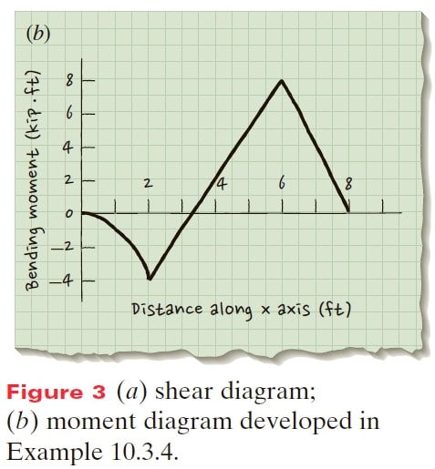
The bending moment is represented by a quadratic equation with a value of −4 kip.ft at x = 2 ft as shown in Figure 3b.
Segment B–C (2 ft ≤ x ≤ 6 ft) and free-body diagram in Figure 2b: Along this segment ω = 0. using (10.6) we get,

V_{y @ C} – V_{y @ B} =  –  \int_{B}^{C}{0 dx}=0

indicating that the shear is a constant between B and C. In fact the shear is a constant 3 kip between B and C.
Now consider the moment by integrating the shear (10.5):

M_{bz @ C} – M_{bz @ B} = \int_{B}^{C}{V_{y} dx} = \int_{2  ft}^{6  ft}{3  kip  dx}  =\left[ (3  kip)x\right]^{6  ft}_{2  ft} =12  kip.ft

This shows that M_{bz} is changing linearly between B and C, and the change is 12 kip.ft. It increases from −4 kip.ft at B to 8 kip.ft at C. This agrees with the previously derived moment diagram in Figure 3b.
Segment C–D (6 ft ≤ x ≤ 8 ft) and free-body diagram in Figure 2c: Along this segment ω = 0. Integrating the distributed load (10.6) gives,

V_{y @ D} – V_{y @ C} =  –  \int_{C}^{D}{0 dx}=0

indicating that the shear is a constant between C and D. The shear diagram indicates a constant −4 kip between C and D.
Finally we consider the moment between C and D using (10.5):

M_{bz @ D} – M_{bz @ C} = \int_{C}^{D}{V_{y} dx} =\int_{6  ft}^{8  ft}{-4  kip  dx}=\left[ (-4  kip)x\right]^{8  ft}_{6  ft} =-8  kip.ft

M_{bz} is changing linearly between C and D, from 8 kip.ft at C to 0 kip.ft at D.
Comment This type of analysis is very useful for checking the values, slopes, and shapes of the shear and bending moment diagrams. Often you don’t need to carry out the integration explicitly, but instead check that the moment is linearly changing if the shear is constant, or the shear is linearly changing if the load is uniformly distributed, etc.