Question 13.5: Consider again a single-axis attitude maneuver depicted in F...

Figure 13.36 shows the reaction-jet control system using the switching signal. There is no way to obtain the system response using analytical methods because the control system is nonlinear; we must use a numerical simulation to obtain the response. We can create a block-diagram simulation of Figure 13.36 using MATLAB’s Simulink software. The Simulink details are not presented here; the interested reader may consult Kluever [4; pp. 162-183, 469-484] for a primer on Simulink.

For this satellite, the magnitude of the control torque is

\left|M_{c}\right|=2 F r=2(400 \mathrm{~N})(2 \mathrm{~m})=1,600 \mathrm{~N}-\mathrm{m}

The constant torque acceleration (magnitude) is \alpha=\left|M_{c}\right| / I_{3}=0.25  \mathrm{rad} / \mathrm{s}^{2}.

First, let us obtain the closed-loop attitude response with dead-zone \varepsilon=0.0004 (\mathrm{rad} / \mathrm{s})^{2}. The switching-signal equation (13.63)

\sigma=-\alpha\phi_{e}-\frac{1}{2}|\dot{\phi}_{e}|\dot{\phi}_{e}        (13.63)

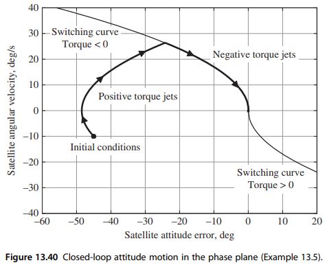
shows that when the angular velocity is very small (\dot{\phi} \approx 0), the switching signal \sigma is in the dead zone when the magnitude of the attitude error is less than \varepsilon / \alpha. For \alpha=0.25  \mathrm{rad} / \mathrm{s}^{2} and \varepsilon=0.0004(\mathrm{rad} / \mathrm{s})^{2}, the jets are inactive when \left|\phi_{e}\right|<0.0016  \mathrm{rad} (or, \left|\phi_{e}\right|<0.1^{\circ} ). Figures 13.37 and 13.38 show the time histories of the closed-loop attitude error \left(\phi_{e}\right) and angular velocity (\dot{\phi}), respectively. Figure 13.37 shows that the attitude error begins at -45^{\circ} and eventually goes to zero at about 4.1 \mathrm{~s}. Figure 13.38 shows that satellite’s angular velocity starts at -10  \mathrm{deg} / \mathrm{s} and steadily increases at a linear rate with time due to the positive torque jets. Positive torque jets are initially used because \sigma>\varepsilon at time t=0 [see Eq. (13.63)]. At time t=2.5 \mathrm{~s}, the switching signal \sigma becomes less than -\varepsilon, and control switches to negative torque jets. At approximately t=4.4 \mathrm{~s}, Figures 13.37 and 13.38 show that the attitude error and attitude rate become small enough so that the switching signal is in the dead zone (i.e., -\varepsilon \leq \sigma \leq \varepsilon) and the jets are turned off. Figure 13.39 shows the time history of the reaction-jet control torque: the switching at t=2.5 \mathrm{~s} is apparent in this figure. At t=4.4 \mathrm{~s}, the jets are turned off because the attitude error and attitude rate are small enough so that |\sigma| \leq \varepsilon. However, at time t=4.9 \mathrm{~s}, the satellite’s attitude angle has drifted away from the reference attitude (note the very small negative attitude rate in Figure 13.38 for t>4.4 \mathrm{~s} ), and consequently \sigma>\varepsilon and a very short positive torque pulse is applied to null the small negative attitude rate. Figure 13.40 shows the closed-loop attitude motion in the phase plane. The initial error state, \phi_{e}=-45^{\circ} and \dot{\phi}_{e}=-10  \mathrm{deg} / \mathrm{s}, is in the positive-torque region, and therefore the switching-signal control law (13.64) correctly calls for positive torque at t=0. Figure 13.40 also shows that the feedback control system correctly switched to negative torque jets when the error states reached the switching curve.

Finally, let us obtain the closed-loop attitude response with a much smaller deadzone \varepsilon=5\left(10^{-8}\right)(\mathrm{rad} / \mathrm{s})^{2}. The closed-loop attitude error and error rate responses are essentially the same as the responses shown in Figures 13.37 and 13.38; that is, the satellite initially exhibits positive angular acceleration (positive torque) between t=0 and t=2.5 \mathrm{~s}, whereupon the torque jets switch to a negative value for 2.5 \leq t \leq 4.4 \mathrm{~s}. The major effect of the tiny dead zone is displayed by the torque history after the satellite has essentially reached its zero-error state. Figure 13.41 shows the reaction-jet control torque history for the case with \varepsilon=5\left(10^{-8}\right)(\mathrm{rad} / \mathrm{s})^{2}. The torque profile matches the control torque for dead zone \varepsilon=0.0004(\mathrm{rad} / \mathrm{s})^{2} (Figure 13.39) until t=4.4 \mathrm{~s}. For t>4.4 \mathrm{~s}, the attitude error \phi_{e} and attitude rate \dot{\phi} are very small (i.e., these states are essentially at the origin of the phase plane), and hence the switching signal \sigma is also very small. However, because \varepsilon is tiny, the switching signal rapidly “drifts” in and out of the dead zone due to very small changes in \phi_{e} and \dot{\phi}. The result is the high-frequency jet switching shown in Figure 13.41 for t>4.4 \mathrm{~s}. This “chattering” control is undesirable because it wastes reaction-jet fuel as it attempts to keep the attitude errors within an unreasonable error threshold.

A final note is in order. In this example, the fixed step size of the numerical integration scheme is \Delta t=0.002 \mathrm{~s}, which implies that the feedback switching signal \sigma is computed 500 times each second (i.e., the sample rate is 1 / \Delta t=500 samples per second = 500 \mathrm{~Hz} ). If the sampling (or feedback measurement) rate is too slow, then the jet switching will be delayed as shown in Figure 13.35. Increasing the sampling rate reduces the switching delay and extraneous control pulses when the error states approach zero. These issues are associated with digital control systems and are beyond the scope of this textbook.