Question 6.PS.2: Coupled Heat and Mass Transfer Let’s now consider the proble...
Coupled Heat and Mass Transfer
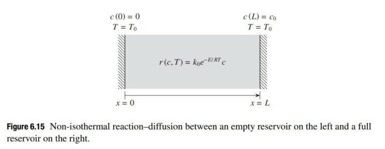
Let’s now consider the problem of calculating the steady state concentration and temperature profile for the system in Fig. 6.15. The concentration of reactant on the left is c(0) = 0, while the concentration on the right is fixed at c(L) = c_0. The steady state mass balance inside the domain is given by
0 = D\frac{d^2c}{dx^2} − r(c, T) (6.6.1)
where
r(c, T) = k_0e^{−E/RT} c (6.6.2)
is the first-order rate of consumption of the reactant. In the latter, k_0 is the preexponential factor, E is the activation energy, R is the ideal gas constant, and T is the temperature. The temperature field also obeys a reaction–diffusion type equation
0 = k\frac{d^2T}{dx^2} + q(c, T) (6.6.3)
where
q(c, T) = r(c, T) \left(\frac{−ΔH_{rxn}}{V}\right) (6.6.4)
is the rate of heat generation inside volume V. We’ll fix the temperature to be at the same value T_0 on both sides of the reactor.
The goal of this problem is to see how the concentration and temperature profiles depend on the Thiele modulus and the activation energy. To keep things interesting, let’s consider endothermic reactions where ΔH_{rxn} > 0.
Learn more on how do we answer questions.
Dimensionless Formulation
Let’s first convert the problem to a dimensionless form with \widetilde{c}= c/c_0, \widetilde{T} = T/T_0, \widetilde{x} = x/L, and the parameter β = E/RT_0. Using these dimensionless variables for the concentration gives us
\frac{Dc_0}{L^2} \frac{d^2\widetilde{c}}{d\widetilde{x}^2 }= k_0e^{−β/\widetilde{T}} c_0\widetilde{c} (6.6.5)
Rearranging the terms gives
\frac{d^2\widetilde{c}}{d\widetilde{x}^2} =\left(\frac{k_0L^2}{D}\right) e^{−β/\widetilde{T}} \widetilde{c} (6.6.6)
The term in brackets is the square of the Thiele modulus,
\phi =\sqrt{\frac{k_0L^2}{D}} (6.6.7)
giving us
\frac{d^2\widetilde{c}}{d\widetilde{x}^2} = \phi^2e^{−β/\widetilde{T}} \widetilde{c} (6.6.8)
The boundary conditions for this equation are
\widetilde{c}(\widetilde{x}= 0) = 0, \widetilde{c}(\widetilde{x} = 1) = 1 (6.6.9)
Applying the same procedure for the temperature gives
\left(\frac{kT_0}{L^2}\right)\frac{ d^2\widetilde{T}}{d\widetilde{x}^2} = k_0e^{−β/\widetilde{T}} \widetilde{c}c_0 \frac{ΔH_{rxn}}{V} (6.6.10)
Rearranging the terms gives
\frac{d^2 \widetilde{T}}{d \widetilde{x}^2} =\left(\frac{k_0c_0 ΔH_{rxn}L^2}{Vk_0T_0}\right) \widetilde{c}e^{−β/\widetilde{T}} (6.6.11)
The term in brackets is a second dimensionless number,
γ =\frac{ k_0c_0 ΔH_{rxn}L^2}{VkT_0} (6.6.12)
which gives us
\frac{d^2\widetilde{T}}{d\widetilde{x}^2 }= γ e^{−β/\widetilde{T}}\widetilde{c} (6.6.13)
The boundary conditions for this equation are
\widetilde{T}(\widetilde{x} = 0) = \widetilde{T}(\widetilde{x} = 1) = 1 (6.6.14)
Numerical Solution
We thus need to solve Eqs. (6.6.8) and (6.6.13) subject to Eqs. (6.6.9) and (6.6.14). To discretize the domain, we use
Δx = \frac{1}{n − 1} (6.6.15)
where n is the number of nodes. We also interlace the variables such that
c_i = y_{2i}−1, T_i = y_{2i} (6.6.16)
For the interior nodes, Eq. (6.6.8) gives
\frac{y_{2i+1} − 2y_{2i−1} + y_{2i−3}}{Δx^2} − \phi ^2y_{2i−1}e^{−β/y_{2i}} = 0 (6.6.17)
for i = 2, … , n − 1. For these same nodes, Eq. (6.6.13) gives
\frac{y_{2i+2} − 2y_{2i} + y_{2i−2}}{Δx^2} − γ y_{2i−1}e^{−β/y_{2i}} = 0 (6.6.18)
The boundary conditions at node i = 1 correspond to
y_1 = 0 (6.6.19)
for concentration and
y_2 − 1 = 0 (6.6.20)
for temperature. Likewise, the boundary conditions at node i = n correspond to
y_{2n−1} − 1 = 0 (6.6.21)
for concentration and
y_{2n} − 1 = 0 (6.6.22)
for temperature.
Equations (6.6.17)–(6.6.22) constitute a system of 2n nonlinear algebraic equations, where we have written all of the equations in the form of the residual. A MATLAB file to calculate the residual is:
1 function R = getR(y,alpha,beta,gamma,n)
2 dx = 1/(n-1);
3 R = zeros(2*n,1);
4 R(1,1) = y(1) - 0;
5 R(2,1) = y(2) - 1;
6 for i = 2:n-1
7 conc_L = (y(2*i+1) -2*y(2*i-1) +y(2*i-3))/dx^2;
8 conc_nL = -alpha*y(2*i-1)*exp(-beta/y(2*i));
9 R(2*i-1,1) = conc_L + conc_nL;
10 T_L = (y(2*i+2) -2*y(2*i) +y(2*i-2))/dx^2;
11 T_nL = -gamma*y(2*i-1)*exp(-beta/y(2*i));
12 R(2*i,1)= T_L + T_nL;
13 end
14 R(2*n-1,1) = y(2*n-1) - 1;
15 R(2*n,1) = y(2*n) - 1;
In the loop for computing the interior node equations, we have broken up the operators into the linear part and the nonlinear part. We use alpha for the square of the Thiele modulus.
We also need the non-zero entries in the Jacobian. For the first row, we have
J_{1,1} = 1 (6.6.23)
from the left boundary condition on concentration (6.6.19). We get the same result for the second row,
J_{2,2} = 1 (6.6.24)
from the left boundary condition on temperature (6.6.20). For the interior nodes, using the local counter i = 2, 3, ... , n − 1, the non-zero entries in the Jacobian are
J_{2i−1,2i−3} = Δx^{−2} (6.6.25)
J_{2i−1,2i−1} = −2Δ x^{−2 }− \phi ^2e^{−β/y_{2i}} (6.6.26)
J_{2i−1,2i} = −\phi ^2 y_{2i−1}e^{−β/y_{2i}} βy^{−2}_{2i} (6.6.27)
J_{2i−1,2i+1} = Δx^{−2} (6.6.28)
for the entries corresponding to the concentration equations (6.6.17) and
J_{2i,2i−2} = Δx^{−2} (6.6.29)
J_{2i,2i−1} = −γ e^−{β/y_{2i}} (6.6.30)
J_{2i,2i} = −2Δ x^{−2} − γ y_{2i−1}e^{−β/y_{2i}} βy^{−2}_{2i} (6.6.31)
J_{2i,2i+2} = Δx^{−2} (6.6.32)
for the entries corresponding to the temperature equations (6.6.18). For the last two rows, we again get
J_{2n−1,2n−1 }= 1 (6.6.33)
from the right boundary condition on concentration (6.6.21) and
J_{2n,2n} = 1 (6.6.34)
from the right boundary condition on temperature (6.6.22). The Jacobian also requires a MATLAB function:
1 function J = getJ(y,alpha,beta,gamma,n)
2 dx = 1/(n-1);
3 dx2 = 1/dx^2;
4 J(1,1) = 1;
5 J(2,2) = 1;
6 for i = 2:n-1
7 r = exp(-beta/y(2*i));
8 J(2*i-1,2*i-3) = dx2;
9 J(2*i-1,2*i-1) = -2*dx2 - alpha*r;
10 J(2*i-1,2*i) = -alpha*y(2*i-1)*r*beta/y(2*i)^2;
11 J(2*i-1,2*i+1) = dx2;
12 J(2*i,2*i-2) = dx2;
13 J(2*i,2*i-1) = - gamma*r;
14 J(2*i,2*i) = -2*dx2 -gamma*y(2*i-1)*r*beta/y(2*i)^2;
15 J(2*i,2*i+2) = dx2;
16 end
17 J(2*n-1,2*n-1) = 1;
18 J(2*n,2*n) = 1;
Since the quantity e^{−β/y_{2i}} appears frequently in the Jacobian, we compute it once on line 7 and use it for the rest of the terms at a given interior node. Also, note that we are doing the counting using the local counter i, which simplifies the bookkeeping. Lines 8–11 implement the entries in the Jacobian for concentration, while lines 12–15 do the same for temperature. Lines 4 and 5 are the left boundary condition, and lines 17 and 18 are the right boundary condition.
Since we are passing parameters for the BVP through the program, we also need to modify the Newton–Raphson program (3.5) to take the inputs:
1 function [x,flag] = nonlinear_newton_raphson(x,tol,paramet)
2 % x = initial guess for x
3 % tol = criteria for convergence
4 % requires function R = getR(x)
5 % requires function J = getJ(x)
6 % flag = 0 if failed, 1 if converged
7 % alpha,beta,gamma,n are parameters from the BVP
8 alpha = paramet(1);
9 beta = paramet(2);
10 gamma = paramet(3)
11 n = paramet(4);
12 R = getR(x,alpha,beta,gamma,n);
13 k = 0; %counter
14 kmax = 100; %max number of iterations allowed
15 while norm(R) > tol
16 J = getJ(x,alpha,beta,gamma,n); %compute Jacobian
17 J = sparse(J);
18 del = -J\R; %Newton Raphson
19 x = x + del; %update x
20 k = k + 1; %update counter
21 R = getR(x,alpha,beta,gamma,n);
22 if k > kmax
23 fprintf('Did not converge.\n')
24 break
25 end
26 end
27 if k > kmax || max(x) == Inf || min(x) == -Inf
28 flag = 0;
29 else
30 flag = 1;
31 end
There are a number of parameters that get passed through the program, so for convenience in our main program they are passed as a vector and then unpacked in lines 8–11 to send to the subfunctions.
To solve the problem, we also need to initialize the vector y. A choice y_i = 1 for this problem is normally good enough to get the solution to converge in three iterations of the Newton–Raphson. When we are done with the calculation, we will normally want to unpack the unknowns into two separate vectors for plotting. We can do this with the following program:
1 function [x,c,T] = extract_coupled_vars(y,n)
2 c = zeros(n,1);
3 T = zeros(n,1);
4 x = linspace(0,1,n);
5 for i = 1:n
6 c(i) = y(2*i-1);
7 T(i) = y(2*i);
8 end
This simple program just loops over the unknown vector y and extracts the odd entries into a new vector c and the even entries into a vector T. For convenience, the program also returns the corresponding entries of the independent variable in the vector x.
Parametric Analysis
We now have a set of MATLAB programs that will solve this nonlinear reaction–diffusion problem given an initial condition and a set of parameters. To look at how the concentration and temperature profiles evolve as a function of the parameters, let’s start with the simplest one. The parameter β is a dimensionless activation temperature relative to the temperature at the boundaries. In other words, it sets the bar for the difficulty in achieving a substantial reaction. It is useful then to consider what happens as β becomes large. In this case, there should be no reaction. Indeed, as we see in Fig. 6.16, the temperature profile becomes flatter and flatter as we increase β, while the concentration profile is approaching the linear one that we would expect in the absence of reaction. From a physical standpoint, the dependence on β is not particularly interesting. From a numerical standpoint, however, this serves as an important check on the accuracy of our solution and whether or not we have any bugs in the code. When you are writing more and more complicated programs, it becomes very useful to test them on cases where you know the answer. Indeed, our next test will bring up a problem with our work so far!
If we make the reaction endothermic and pick a relatively small activation temperature, say β = 0.01, we see in Fig. 6.16 that the temperature gets very low without much reaction. This particular example shows a very strong coupling between the transport of heat and species. There is also an analogy with the case of a stiff system of IVPs that we discussed in Section 4.8.2. For stiff IVPs, we have a wide separation of eigenvalues and we need to keep the time step small with respect to the largest eigenvalue so that we have numerical stability. In the case of coupled BVPs, it is possible to have one of the dependent variables change much more rapidly than the other dependent variables. The most rapidly changing dependent variable, in this case the temperature, sets the spatial discretization size Δx that we need to avoid large errors in the solution. Since the equations are coupled, errors in the solution for the temperature will be transmitted to the concentration through the reaction term. The difference between BVPs and IVPs is that there is no equivalent of the stability condition for a BVP – we will obtain a solution to the BVP for large Δx, but it will just be inaccurate. It is unlikely that the solution will diverge, although it is always possible that a nonlinear system will find an unphysical solution due to discretization error.
Let’s consider a more interesting case where we consider the balance between reaction and diffusion embodied in the Thiele modulus. If \phi= 0, then there should be no reaction. Thus, we would expect a small Thiele modulus to be the same as the large β case in Fig. 6.16. This is obviously not the case in Fig. 6.17!
The question we need to answer is whether this is due to a bug in our program, an unphysical solution caused by a bad guess, or some other problem. In general, this is a very difficult question to answer. We normally look at known cases to test out the code before considering other problems where we don’t know the answer. In the case of no reaction, the coupling in Eqs. (6.6.1) and (6.6.3) should disappear – the concentration should be a linear profile between the reservoirs and the temperature should be uniform. The solution we see in Fig. 6.17 gives us a clue to the source of the problem. The concentration profile looks correct, with a perfectly linear solution between the two reservoirs. So the problem must be in the temperature equations. If we look back at the definition of the parameter γ in Eq. (6.6.12), we see that it could be written in the form
γ =\left(\frac{k_0L^2}{D}\right)\left(\frac{Dc_0 H_{rxn}}{VkT_0}\right) (6.6.35)
where the first term in brackets is the square of the Thiele modulus. Thus, we are not actually free to set the parameters φ and γ independently – if we wanted to set the Thiele modulus to zero and eliminate the reaction, we would have needed the second term to be infinitely large to lead to a non-zero limiting value. This is physically unrealistic.
We put in a deliberate trap in this problem in the definition of γ to bring up an important point about non-dimensionalization of a problem, especially a complicated one that requires numerical methods. This is a powerful approach, but you should be careful that your dimensionless parameters are indeed independent. If you look back to the non-isothermal CSTR problem in Section 5.7, you will see that we were careful to separate out the coefficient for the reactive contribution to the temperature equation into the Thiele modulus and Prater number, which avoids mixing different effects. Fortunately, we were able to use our numerical analysis to find the shortcoming in the problem formulation that we used here.

