Question 14.11: Design of a New Geometrically Similar Pump After graduation,...
Design of a New Geometrically Similar Pump
After graduation, you work for a pump manufacturing company. One of your company’s best-selling products is a water pump, which we shall call pump A. Its impeller diameter is D_A = 6.0 cm, and its performance data when operating at \dot{n}_{ A }=1725 rpm \left(\omega_{ A }=180.6 rad / s \right) are shown in Table 14–2. The marketing research department is recommending that the company design a new product, namely, a larger pump (which we shall call pump B) that will be used to pump liquid refrigerant R-134a at room temperature. The pump is to be designed such that its best efficiency point occurs as close as possible to a volume flow rate of \dot{V}_{ B }=2400 cm ^3 / s and at a net head of H_B = 450 cm (of R-134a). The chief engineer (your boss) tells you to perform some preliminary analyses using pump scaling laws to determine if a geometrically scaled-up pump could be designed and built to meet the given requirements. (a) Plot the performance curves of pump A in both dimensional and dimensionless form, and identify the best efficiency point. (b) Calculate the required pump diameter D_B, rotational speed \dot{n}_{ B} , and brake horsepower bhp_B for the new product.
TABLE 14–2
Manufacturer’s performance data for a water pump operating at 1725 rpm and room temperature (Example 14–11)*
| \eta_{\text {pump }}, \% | H, cm | \dot{ V }, cm ^3 / s |
| 32 | 180 | 100 |
| 54 | 185 | 200 |
| 70 | 175 | 300 |
| 79 | 170 | 400 |
| 81 | 150 | 500 |
| 66 | 95 | 600 |
| 38 | 54 | 700 |
* Net head is in centimeters of water.
Learn more on how we answer questions.
(a) For a given table of pump performance data for a water pump, we are to plot both dimensional and dimensionless performance curves and identify the BEP. (b) We are to design a new geometrically similar pump for refrigerant R-134a that operates at its BEP at given design conditions.
Assumptions 1 The new pump can be manufactured so as to be geometrically similar to the existing pump. 2 Both liquids (water and refrigerant R-134a) are incompressible. 3 Both pumps operate under steady conditions.
Properties At room temperature (20°C), the density of water is \rho_{water} = 998.0 kg/m^3 and that of refrigerant R-134a is \rho_{R-134a} = 1226 kg/m^3.
Analysis (a) First, we apply a second-order least-squares polynomial curve fit to the data of Table 14–2 to obtain smooth pump performance curves. These are plotted in Fig. 14–76, along with a curve for brake horsepower, which is obtained from Eq. 14–5. A sample calculation, including unit conversions, is shown in Eq. 1 for the data at \dot{V}_{ A }=500 cm ^3 / s , which is approximately the best efficiency point:
\eta_{\text {pump }}=\frac{\dot{W}_{\text {water horsepower }}}{\dot{W}_{\text {shaft }}}=\frac{\dot{W}_{\text {water horsepower }}}{\text { bhp }}=\frac{\rho g \dot{V} H}{\omega T _{\text {shaft }}} (14.5)
bhp _{ A }=\frac{\rho_{\text {water }} g \dot{V}_{ A } H_{ A }}{\eta_{\text {pump }, A }} =\frac{\left(998.0 kg / m ^3\right)\left(9.81 m / s ^2\right)\left(500 cm ^3 / s \right)(150 cm )}{0.81}\left(\frac{1 m }{100 cm }\right)^4\left(\frac{ W \cdot s }{ kg \cdot m ^2 / s ^2}\right)
= 9.07 W (1)
Note that the actual value of bhpA plotted in Fig. 14–76 at \dot{V}_{ A }=500 cm ^3 / s differs slightly from that of Eq. 1 due to the fact that the least-squares curve fit smoothes out scatter in the original tabulated data.
Next we use Eqs. 14–30 to convert the dimensional data of Table 14–2 into nondimensional pump similarity parameters. Sample calculations are shown in Eqs. 2 through 4 at the same operating point as before (at the approximate location of the BEP). At \dot{V}_{ A }=500 cm ^3 / s the capacity coefficient is approximately
C_H=\text { Head coefficient }=\frac{g H}{\omega^2 D^2}
C_Q=\text { Capacity coefficient }=\frac{\dot{V}}{\omega D^3} (14.30)
C_P=\text { Power coefficient }=\frac{ bhp }{\rho \omega^3 D^5}
C_Q=\frac{\dot{V}}{\omega D^3}=\frac{500 cm ^3 / s }{(180.6 rad / s )(6.0 cm )^3}=0.0128 (2)
The head coefficient at this flow rate is approximately
C_H=\frac{g H}{\omega^2 D^2}=\frac{\left(9.81 m / s ^2\right)(1.50 m )}{(180.6 rad / s )^2(0.060 m )^2}=0.125 (3)
Finally, the power coefficient at \dot{V}_{ A }=500 cm ^3 / s is approximately
C_P=\frac{ bhp }{\rho \omega^3 D^5}=\frac{9.07 W }{\left(998 kg / m ^3\right)(180.6 rad / s )^3(0.060 m )^5}\left(\frac{ kg \cdot m ^2 / s ^2}{ W \cdot s }\right)=0.00198 (4)
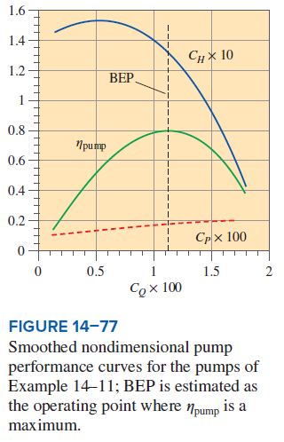
These calculations are repeated (with the aid of a spreadsheet) at values of \dot{V}_{ A } between 100 and 700 cm³/s. The curve-fitted data are used so that the normalized pump performance curves are smooth; they are plotted in Fig. 14–77. Note that \eta_{\text {pump }} is plotted as a fraction rather than as a percentage. In addition, in order to fit all three curves on one plot with a single ordinate, and with the abscissa centered nearly around unity, we have multiplied C_Q by 100, C_H by 10, and C_P by 100. You will find that these scaling factors work well for a wide range of pumps, from very small to very large. A vertical line at the BEP is also sketched in Fig. 14–77 from the smoothed data. The curve-fitted data yield the following nondimensional pump performance parameters at the BEP:
C_Q^*=0.0112 C_H^*=0.133 C_P^*=0.00184 \eta_{\text {pump }}^*=0.812 (5)
(b) We design the new pump such that its best efficiency point is homologous with the BEP of the original pump, but with a different fluid, a different pump diameter, and a different rotational speed. Using the values identified in Eq. 5, we use Eqs. 14–30 to obtain the operating conditions of the new pump. Namely, since both \dot{V}_{ B } and H_B are known (design conditions), we solve simultaneously for D_B and \omega_{ B } .
After some algebra in which we eliminate \omega_{ B } , we calculate the design diameter for pump B,
D_{ B }=\left(\frac{\dot{V}_{ B }^2 C_H^*}{\left(C_Q^*\right)^2 g H_{ B }}\right)^{1 / 4}=\left(\frac{\left(0.0024 m ^3 / s \right)^2(0.133)}{(0.0112)^2\left(9.81 m / s ^2\right)(4.50 m )}\right)^{1 / 4}= 0 . 1 0 8 m (6)
In other words, pump A needs to be scaled up by a factor of D_B/D_A = 10.8 cm/6.0 cm = 1.80. With the value of D_B known, we return to Eqs. 14–30 to solve for \omega_B, the design rotational speed for pump B,
\omega_{ B }=\frac{\dot{V}_{ B }}{\left(C_Q{ }^*\right) D_{ B }^3}=\frac{0.0024 m ^3 / s }{(0.0112)(0.108 m )^3}=168 rad / s \quad \rightarrow \quad \dot{n}_{ B }= 1 6 1 0 \mathrm { rpm } (7)
Finally, the required brake horsepower for pump B is calculated from Eqs. 14–30, bhp _{ B }=\left(C_P^*\right) \rho_{ B } \omega_{ B }^3 D_{ B }^5
=(0.00184)\left(1226 kg / m ^3\right)(168 rad / s )^3(0.108 m )^5\left(\frac{ W \cdot s }{ kg \cdot m ^2 / s ^2}\right)= 1 6 0 W (8)
An alternative approach is to use the affinity laws directly, eliminating some intermediate steps. We solve Eqs. 14–38a and b for D_B by eliminating the ratio \omega_B/\omega_A.
We then plug in the known value of D_A and the curve-fitted values of \dot{V}_A and H_A at the BEP (Fig. 14–78). The result agrees with those calculated before. In a similar manner we can calculate \omega_B and bhp_B.
\frac{\dot{V}_{ B }}{\dot{V}_{ A }}=\frac{\omega_{ B }}{\omega_{ A }}\left(\frac{D_{ B }}{D_{ A }}\right)^3 (14.38a)
Discussion Although the desired value of \omega_B has been calculated precisely, a practical issue is that it is difficult (if not impossible) to find an electric motor that rotates at exactly the desired rpm. Standard single-phase, 60-Hz, 120-V AC electric motors typically run at 1725 or 3450 rpm. Thus, we may not be able to meet the rpm requirement with a direct-drive pump. Of course, if the pump is belt-driven or if there is a gear box or a frequency controller, we can easily adjust the configuration to yield the desired rotation rate. Another option is that since \omega_B is only slightly smaller than \omega_A, we drive the new pump at standard motor speed (1725 rpm), providing a somewhat stronger pump than necessary.
The disadvantage of this option is that the new pump would then operate at a point not exactly at the BEP.