Question 21.1: Determine the shear flow distribution in the web of the tape...
Determine the shear flow distribution in the web of the tapered beam shown in Fig. 21.2, at a section midway along its length. The web of the beam has a thickness of 2 mm and is fully effective in resisting direct stress. The beam tapers symmetrically about its horizontal centroidal axis and the cross-sectional area of each flange is 400 mm².

Learn more on how we answer questions.
The internal bending moment and shear load at the section AA produced by the externally applied load are, respectively
M_x=20 \times 1=20 \mathrm{kN} \mathrm{m} \quad S_y=-20 \mathrm{kN}
The direct stresses parallel to the z axis in the flanges at this section are obtained either from Eqs (16.18) or (16.19) in which M_y=0 \text { and } I_{x y}=0. Thus, from Eq. (16.18)
\sigma_z=\frac{M_x\left(I_{y y} y-I_{x y} x\right)}{I_{x x} I_{y y}-I_{x y}^2}+\frac{M_y\left(I_{x x} x-I_{x y} y\right)}{I_{x x} I_{y y}-I_{x y}^2} (16.18)
\sigma_z=\frac{M_x\left(I_{y y} y-I_{x y} x\right)}{I_{x x} I_{y y}-I_{x y}^2}+\frac{M_y\left(I_{x x} x-I_{x y} y\right)}{I_{x x} I_{y y}-I_{x y}^2} (16.19)
\sigma_z=\frac{M_x y}{I_{x x}} (i)
in which
I_{x x}=2 \times 400 \times 150^2+2 \times 300^3 / 12
i.e.
I_{x x}=22.5 \times 10^6 \mathrm{~mm}^4
Hence
The components parallel to the z axis of the axial loads in the flanges are therefore
P_{z, 1}=-P_{z, 2}=133.3 \times 400=53320 \mathrm{~N}
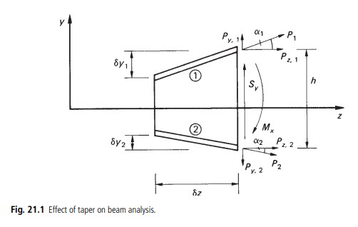
The shear load resisted by the beam web is then, from Eq. (21.5)
S_{y, w}=S_y-P_{z, 1} \frac{\delta y_1}{\delta z}-P_{z, 2} \frac{\delta y_2}{\delta z} (21.5)
S_{y, w}=-20 \times 10^3-53320 \frac{\delta y_1}{\delta z}+53320 \frac{\delta y_2}{\delta z}in which, from Figs 21.1 and 21.2, we see that
\frac{\delta y_1}{\delta z}=\frac{-100}{2 \times 10^3}=-0.05 \quad \frac{\delta y_2}{\delta z}=\frac{100}{2 \times 10^3}=0.05Hence
S_{y, w}=-20 \times 10^3+53320 \times 0.05+53320 \times 0.05=-14668 \mathrm{~N}The shear flow distribution in the web follows either from Eq. (21.6) or Eq. (21.7) and is (see Fig. 21.2(b))
q_s=-\frac{S_{y, w}}{I_{x x}}\left(\int_0^s t_{\mathrm{D}} y \mathrm{~d} s+B_1 y_1\right) (21.6)
q_s=-\frac{S_{y, w}}{I_{x x}}\left(\int_0^s t_{\mathrm{D}} y \mathrm{~d} s+B_2 y_2\right) (21.7)
q_{12}=\frac{14668}{22.5 \times 10^6}\left(\int_0^s 2(150-s) \mathrm{d} s+400 \times 150\right)i.e.
q_{12}=6.52 \times 10^{-4}\left(-s^2+300 s+60000\right) (ii)
The maximum value of q_{12} occurs when s = 150 mm and q_{12} (max) = 53.8 N/mm. The values of shear flow at points 1 (s = 0) and 2 (s = 300 mm) are q_1 = 39.1 N/mm and q_2 = 39.1 N/mm; the complete distribution is shown in Fig. 21.3