Question 11.15.11: Determine the state space representation of the continuous-t...
Determine the state space representation of the continuous-time system with transfer function
H(s)=\frac{s^2+2}{s^3+s^2+4s+2} .
Compute and plot in the time interval 0 ≤ t ≤ 20 the impulse response and the step response of the system according to its state representation. Also, calculate the system response to the input signal
\upsilon (t)= \begin{cases} 2t, & 0\leq t\leq 2 \\ 8-2t, & 2<t\leq 4\end{cases}Finally, compute and plot the state process when the applied input signal is the Dirac function δ(t) and when the applied input signal is \upsilon(t).
num=[1 0 2];
den=[1 1 4 2];
[A,B,C,D]=tf2ss(num,den)
A = -1 -4 -2
1 0 0
0 1 0
B = 1
0
0
C = 1 0 2
D = 0
The SS model of the system is
x(t)= \left[\begin{matrix} -1 & -4 & -2 \\ 1 & 0 & 0 \\ 0 & 1 & 0 \end{matrix} \right] x(t)+\left[\begin{matrix} 1 \\ 0 \\ 0 \end{matrix} \right] \upsilon (t)
y(t) = [1\ \ \ \ 0\ \ \ \ 2] \upsilon (t)
sys=ss(A,B,C,D);
t=0:.1:20;
h=impulse(sys,t);
plot(t,h)
legend('Impulse response')
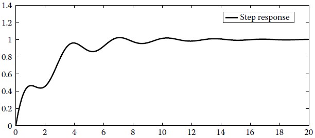
s=step(sys,t);
plot(t,s)
legend('Step response')
t1=0:.1:2;
t2=2.1:.1:4;
t3=4.1:.1:20;
t=[t1 t2 t3];
v1=2*t1;
v2=8-2*t2;
v3=zeros(size(t3));
v=[v1 v2 v3];
y=lsim(sys,v,t);
plot(t,y);
legend('System response')
[y,t,x]=impulse(sys,t);
plot(t,x(:,1),t,x(:,2),'+',t,x(:,3),'o')
legend('x_1(t)','x_2(t)','x_3(t)')
title('State trajectories–input signal \delta(t)')
[y,t,x]=lsim(sys,v,t)
plot(t,x(:,1),t,x(:,2),':+',t,x(:,3),':o')
legend('x_1(t)','x_2(t)','x_3(t)')
title('State trajectories –input signal x(t))')
Notice that the state of the system depends on the applied input signal.