Question 6.1: Determining Estimated S-N Diagrams for Ferrous Materials Pro...
Determining Estimated S-N Diagrams for Ferrous Materials
Problem Create an estimated S-N diagram for a steel bar and define its equations. How many cycles of life can be expected if the alternating stress is 100 MPa?
Given The S_{ut} has been tested at 600 MPa. The bar is 150 mm square and has a hot-rolled finish. The operating temperature is 500°C maximum. The loading will be fully reversed bending.
Assumptions Infinite life is required and is obtainable since this ductile steel will have an endurance limit. A reliability factor of 99.9% will be used.
Learn more on how we answer questions.
1 Since no endurance-limit or fatigue strength information is given, we will estimate S_e{ }^{\prime} based on the ultimate strength using equation 6.5a (p. 330).
\text { steels : } \quad\left\{\begin{array}{ll} S_{e^{\prime}} \cong 0.5 S_{u t} & \text { for } S_{u t}<200 kpsi (1400 MPa ) \\ S_{e^{\prime}} \cong 100 kpsi (700 MPa ) & \text { for } S_{u t} \geq 200 kpsi (1400 MPa ) \end{array}\right\} (6.5a)
S_{e^{\prime}} \cong 0.5 S_{u t}=0.5(600)=300 MPa (a)
2 The loading is bending so the load factor from equation 6.7a is
\begin{array}{ll} \text { bending: } & C_{\text {load }}=1 \\ \text { axial loading: } & C_{\text {load }}=0.70 \end{array} (6.7a)
C_{load} = 1.0 (b)
3 The part is larger than the test specimen and is not round, so an equivalent diameter based on its 95% stressed area (A_{95} ) must be determined and used to find the size factor. For a rectangular section in nonrotating bending loading, the A_{95 } area is defined in Figure 6- 25c (p. 332) and the equivalent diameter is found from equation 6.7d (p. 331):
d_{\text {equiv }}=\sqrt{\frac{A_{95}}{0.0766}} (6.7d)
\begin{aligned} A_{95} &=0.05 b h=0.05(150)(150)=1125 mm ^2 \\ d_{\text {equiv }} &=\sqrt{\frac{A_{95}}{0.0766}}=\sqrt{\frac{1125 mm ^2}{0.0766}}=121.2 mm \end{aligned} (c)
and the size factor is found for this equivalent diameter from equation 6.7b (p. 331):
\text {for} d \leq 0.3 \text {in} (8 mm) : \quad C_{\text {size }}=1 \\ \text {for} 0.3 \text {in} \lt d \leq 10 \text {in} : \quad C_{\text {size }}=0.869 d^{-0.097} \\ \text {for} 8 mm \lt d \leq 250 mm : \quad C_{\text {size }}=1.189 d^{-0.097} (6.7b)
C_{\text {size }}=1.189(121.2)^{-0.097}=0.747 (d)
4 The surface factor is found from equation 6.7e (p. 333) and the data in Table 6-3 for the specified hot-rolled finish.
C_{\text {surf }} \equiv A\left(S_{\text {ut }}\right)^b \quad \text { if } C_{\text {surf }}>1.0 \text {, set } C_{\text {surf }}=1.0 (6.7e)
C_{\text {surf }}=A S_{u t}^b=57.7(600)^{-0.718}=0.584 (e)
5 The temperature factor is found from equation 6.7f (p. 335):
\text {for} T \leq 450^\circ C (840^\circ F) : \quad C_{\text {temp }}=1\\ \text {for} 450^\circ C \lt T \leq 550^\circ C : \quad C_{\text {temp }}=1-0.0058(T-450)\\ \text {for} 840^\circ F \lt T\leq 1020^\circ F : C_{\text {temp }}=1-0.0032(T-840) (6.7f)
C_{\text {temp }}=1-0.0058(T-450)=1-0.0058(500-450)=0.71 (f)
6 The reliability factor is taken from Table 6-4 (p. 335) for the desired 99.9% and is
C_{\text {reliab }}=0.753 (g)
7 The corrected endurance limit S_{e} can now be calculated from equation 6.6 (p. 330):
\begin{array}{l} S_e=C_{\text {load }} C_{\text {size }} C_{\text {surf }} C_{\text {temp }} C_{\text {reliab }} S_{e^{\prime}} \\ S_f=C_{\text {load }} C_{\text {size }} C_{\text {surf }} C_{\text {temp }} C_{\text {reliab }} S_f^{\prime} \end{array} (6.6)
\begin{aligned} S_e &=C_{\text {load }} C_{\text {size }} C_{\text {surf }} C_{\text {temp }} C_{\text {reliab }} S_{e^{\prime}} \\ &=1.0(0.747)(0.584)(0.71)(0.753)(300) \\ S_e &=70 MPa \end{aligned} (h)
8 To create the S-N diagram, we also need a number for the estimated strength S_{m} at 10³ cycles based on equation 6.9 (p. 337) for bending loading.
\text {bending :} \quad \quad S_m=0.9 S_{u t} \\ \text {axial loading :} \quad \quad S_m=0.75 S_{u t} (6.9)
S_m=0.90 S_{u t}=0.90(600)=540 MPa (i)
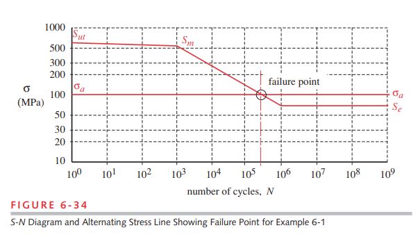
9 The estimated S-N diagram is shown in Figure 6-34 with the above values of S_{m} and S_{e}. The expressions of the two lines are found from equations 6.10a through 6.10c (p. 338) assuming that S_{e} begins at 10^{6} cycles.
S(N)=a N^b (6.10a)
\begin{array}{c} b=-\frac{1}{3} \log \left\lgroup\frac{S_m}{S_e}\right\rgroup =-\frac{1}{3} \log \left\lgroup\frac{540}{70}\right\rgroup =-0.295765 \\ \log (a)=\log \left(S_m\right)-3 b=\log [540]-3(-0.295765): \quad a=4165.707 \end{array} (j)
\begin{array}{ll} S(N)=a N^b=4165.707 N^{-0.295765} MPa & 10^3 \leq N \leq 10^6 \\ S(N)=S_e=70 MPa & N>10^6 \end{array} (k)
10 The number of cycles of life for any alternating stress level can now be found from equations (k). For the stated stress level of 100 MPa, we get
\begin{aligned} 100 &=4165.707 N^{-0.295765} \quad 10^3 \leq N \leq 10^6 \\ \log 100 &=\log 4165.707-0.295765 \log N \\ 2 &=3.619689-0.295765 \log N \\ \log N &=\frac{2-3.619689}{-0.295765}=5.476270 \\ N &=10^{5.476270}=3.0 E 5 \text { cycles } \end{aligned} (l)
Figure 6-34 shows the intersection of the alternating stress line with the failure line at N = 3E5 cycles.
11 The files EX06-01 are on the CD-ROM.
| Table 6-3 Coefficients for Surface-Factor Equation 6.7e Source: Shigley and Mischke, Mechanical Engineering Design, 5th ed., McGrawHill, New York, 1989, p. 283 with permission | ||||
| For S_{ut} in MPa use | For S_{ut} in kpsi
(not psi) use |
|||
| Surface Finish | A | b | A | b |
| Ground | 1.58 | –0.085 | 1.34 | –0.085 |
| Machined or cold-rolled | 4.51 | –0.265 | 2.7 | –0.265 |
| Hot-rolled | 57.7 | –0.718 | 14.4 | –0.718 |
| As-forged | 272 | –0.995 | 39.9 | –0.995 |
| Table 6-4 Reliability Factors for S_{d} = 0.08 \mu |
|
| Reliability % | C_{reliab} |
| 50 | 1.000 |
| 90 | 0.897 |
| 95 | 0.868 |
| 99 | 0.814 |
| 99.9 | 0.753 |
| 99.99 | 0.702 |
| 99.999 | 0.659 |
| 99.9999 | 0.620 |