Question 13.6: Develop a spectrum between yield strength reduction factor a...
Develop a spectrum between yield strength reduction factor and period for the ground motion of Example 13.5. Also draw inelastic response spectrum on a log-log scale.
Learn more on how we answer questions.
| Ground Motion | |
| Max. Acceleration | 1 g |
| Max. Velocity | 90 cm/s |
| Max. Displacement | 60 cm |
Equations (13.30) can be re-written as follows:
F_{y}=\frac{\text{Elastic strength}}{R} (13.30a)
F_{y}=kx_{y}=m\omega ^{2}_{n}x_{y}=mA_{y}=\frac{\mathrm{w}}{g} A_{y} (13.30b)
R=\frac{\text{Elastic strength}}{\text{Yield strength}}
The reduction factors for different regions were given by Equation (13.31). From the tripartite spectra generated in Figure 13.31, determine the periods T_{c} and {T_{c}}^{\prime}. The relation between yield strength reduction factor R and period T for different ductility ratio is shown in Table 13.3 and log-log graph Figure 13.32. The period T_{c} is 0.5 sec while {T_{c}}^{\prime} values are highlighted in Table 13.3.
Knowing the elastic spectra for µ = 1, the acceleration ordinate for a given ductility can be computed using the following equation:
A^{\prime}=\frac{A}{\sqrt{2\mu -1} } (13.34c)
where A = elastic acceleration spectrum ordinate
R = 1 for T < T_{A} (13.31a)
R=(2\mu -1)^{\gamma /2} for T_{A} < T < T_{B} (13.31b)
R=(2\mu -1)^{0.5} for T_{B}< T <{T_{C}}^{\prime} (13.31c)
R= (T/T_{C})\mu for {T_{C}}^{\prime} < T < T_{C} (13.31d)
R = µ for T >T_{C} (13.31e)
Table 13.3 Relation between R and T for a Given Ductility μ
| Ductility µ | |||||||
| µ = 1.5 | µ = 2 | µ = 4 | µ = 6 | ||||
| R | T | R | T | R | T | R | T |
| 1 | 0.01 | 1 | 0.01 | 1 | 0.01 | 1 | 0.01 |
| 1 | 0.03 | 1 | 0.03 | 1 | 0.03 | 1 | 0.03 |
| 1.41 | 0.125 | 1.73 | 0.125 | 2.64 | 0.125 | 3.31 | 0.125 |
| 1.41 | 0.45 | 1.73 | 0.43 | 2.64 | 0.33 | 3.31 | 0.28 |
| 1.41 | 0.47 | 1.8 | 0.45 | 3.6 | 0.45 | 5.4 | 0.45 |
| 1.5 | 0.5 | 2 | 0.5 | 4 | 0.5 | 6 | 0.5 |
| 1.5 | 10 | 2 | 10 | 4 | 10 | 6 | 10 |
| 1.5 | 33 | 2 | 33 | 4 | 33 | 6 | 33 |
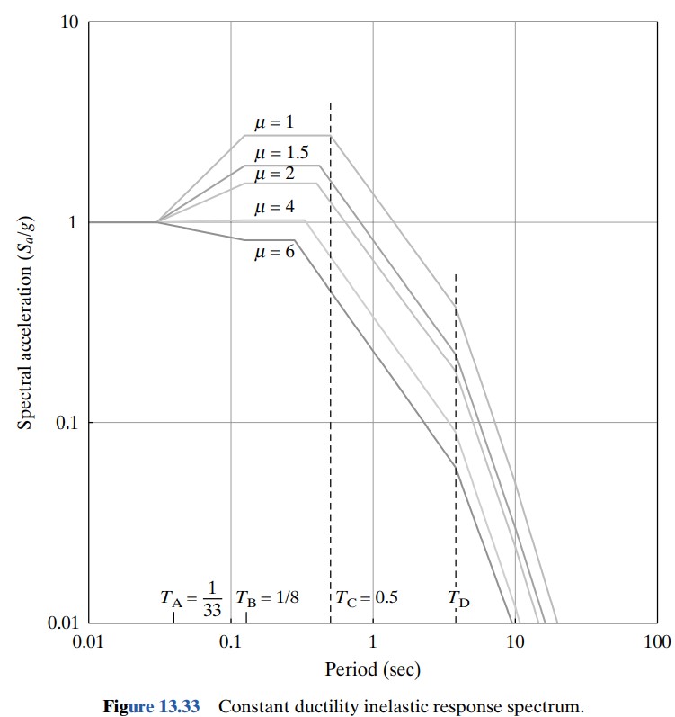
The relation between acceleration S_{a} and period T for different ductility µ is shown in Table 13.4 and in log-log graph in Figure 13.33. The values in the table are shown only upto μ = 2. Similar calculations can be done for other values of μ.
Table 13.4 Relation between S_{a} and T for Different Ductility μ
| µ = 1 | µ = 1.5 | µ = 2 | |||||
| S_{a}/g | T(sec) | R | S_{a}/g | T(sec) | R | S_{a}/g | |
| 1 | 0.01 | 1 | 1 | 0.01 | 1 | 1 | 0.01 |
| 1 | 0.03 | 1 | 1 | 0.03 | 1 | 1 | 0.03 |
| 2.71 | 0.125 | 1.41 | 1.92 | 0.125 | 1.73 | 1.56 | 0.125 |
| 2.71 | 0.5 | 1.41 | 1.92 | 0.47 | 1.73 | 1.56 | 0.43 |
| 0.38 | 4 | 1.5 | 0.25 | 4 | 2 | 0.19 | 4 |
| 0.05 | 10 | 1.5 | 0.03 | 10 | 2 | 0.03 | 10 |
| 0.003 | 33 | 1.5 | 0 | 33 | 2 | 0 | 33 |