Question 10.3: Draw the Bode log-magnitude and phase plots of G(s) for the ...
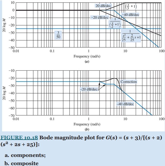
Draw the Bode log-magnitude and phase plots of G(s) for the unity-feedback system shown in Figure 10.10, where G(s) = (s + 3)/[(s + 2) (s² + 2s + 25)].

Learn more on how we answer questions.
We first convert G(s) to show the normalized components that have unity low-frequency gain. The second-order term is normalized by factoring out ω^{2}_{n} , forming
\frac{s²}{ω^{2}_{n}} + \frac{2ζ}{ω_{n}} s + 1 (10.35)
Thus,
G(s) = \frac{3}{(2)(25)} \frac{(\frac{s}{3} + 1 )}{(\frac{s}{2} + 1 ) (\frac{s²}{25} + \frac{2}{25} s + 1 )} = \frac{3}{50} \frac{(\frac{s}{3} + 1 )}{(\frac{s}{2} + 1 ) (\frac{s²}{25} + \frac{2}{25} s + 1 )} (10.36)
The Bode log-magnitude diagram is shown in Figure 10.18(b) and is the sum of the individual first- and second-order terms of G(s) shown in Figure 10.18(a). We solve this problem by adding the slopes of these component parts, beginning and ending at the appropriate frequencies. The results are summarized in Table 10.6, which can be used to obtain the slopes. The low-frequency value for G(s), found by letting s = 0, is 3/50, or −24.44 dB. The Bode magnitude plot starts out at this value and continues until the first break frequency at 2 rad/s. Here the pole at −2 yields a −20 dB/decade slope downward until the next break at 3 rad/s. The zero at −3 causes an upward slope of +20 dB/decade, which, when added to the previous −20 dB/decade curve, gives a net slope of 0. At a frequency of 5 rad/s, the second-order term initiates a −40 dB/decade downward slope, which continues to infinity.
TABLE 10.6 Magnitude diagram slopes for Example 10.3
| Frequency (rad/s) | ||||
| Description | 0.01 (Start: Plot) |
2 (Start: Pole at −2) |
3 (Start: Zero at −3) |
5 (Start: ω_{n} = 5) |
| Pole at −2 | 0 | −20 | −20 | −20 |
| Zero at −3 | 0 | 0 | 20 | 20 |
| ω_{n} = 5 | 0 | 0 | 0 | −40 |
| Total slope (dB/dec) |
0 | −20 | 0 | −40 |
The correction to the log-magnitude curve due to the underdamped second-order term can be found by plotting a point −20 log 2ζ above the asymptotes at the natural frequency. Since ζ = 0.2 for the second-order term in the denominator of G(s), the correction is 7.96 dB. Points close to the natural frequency can be corrected by taking the values from the curves of Figure 10.16.
We now turn to the phase plot. Table 10.7 is formed to determine the progression of slopes on the phase diagram. The first-order pole at −2 yields a phase angle that starts at 0° and ends at −90° via a −45°/decade slope starting a decade below its break frequency and ending a decade above its break frequency. The first-order zero yields a phase angle that starts at 0° and ends at +90° via a +45°/decade slope starting a decade below its break frequency and ending a decade above its break frequency. The second-order poles yield a phase angle that starts at 0° and ends at −180° via a −90°/decade slope starting a decade below their natural frequency ( ω_{n} = 5) and ending a decade above their natural frequency. The slopes, shown in Figure 10.19(a), are summed over each frequency range, and the final Bode phase plot is shown in Figure 10.19(b).
TABLE 10.7 Phase diagram slopes for Example 10.3
| Frequency (rad/s) | ||||||
| Description | 0.2 (Start: Pole at −2) |
0.3 (Start: Zero at −3) |
0.5 (Start: ω_{n} at −5) |
20 (End: Pole at −2) |
30 (End: Zero at −3) |
50 (End: ω_{n} = 5) |
| Pole at −2 | −45 | −45 | −45 | 0 | ||
| Zero at −3 | 45 | 45 | 45 | 0 | ||
| ω_{n} = 5 | −90 | −90 | −90 | 0 | ||
| Total slope (dB/dec) |
−45 | 0 | −90 | −45 | −90 | 0 |
Students who are using MATLAB should now run ch10apB1 in Appendix B. You will learn how to use MATLAB to make Bode plots and list the points on the plots. This exercise solves Example 10.3 using MATLAB.