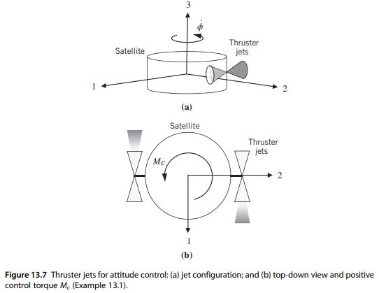
Question 13.1: Figure 13.7 shows a cylindrical-shaped satellite equipped wi...
Figure 13.7 shows a cylindrical-shaped satellite equipped with two pairs of reaction jets (thrusters). Firing the two jet pairs as shown in Figure 13.7b imparts a positive control torque M_{c} about the 3 axis (of course, firing the opposite jet pairs produces a negative torque). Suppose the satellite’s moment of inertia about the 3 axis is I_{3}= 1,000 \mathrm{~kg}-\mathrm{m}^{2}. The jet pairs are located 1.5 \mathrm{~m} from the 3 axis. Assuming that each jet can be throttled to produce variable thrust up to a maximum value of 20 \mathrm{~N}, design a feedback controller that provides a fast, well-damped response to a constant attitude-rotation command of \pi rad (i.e., a 180^{\circ} attitude maneuver). We will assume that the satellite is initially at rest [\dot{\phi}(0)=0] with zero attitude angle \phi(0)=0.
Learn more on how we answer questions.
Figure 13.8 shows the closed-loop attitude control system for this example (it is essentially the same as Figure 13.5 with the satellite dynamics represented by a single transfer function). Let us begin by investigating an extremely simple controller strategy known as proportional control, that is, the control torque is proportional to the attitude error:
\text { Proportional control: } M_{c}=K_{P} \phi_{e} (13.19)
where K_{P} is called the proportional gain. In this case, K_{P} has units of torque/angular displacement or \mathrm{N}-\mathrm{m} / \mathrm{rad}. For this fictitious example, we have assumed that each thruster can be throttled from zero to 20 \mathrm{~N}, and therefore the maximum control torque magnitude is (2)(20 \mathrm{~N})(1.5 \mathrm{~m})=60 \mathrm{~N}-\mathrm{m} (recall that the jets are fired in pairs and that each jet has a moment arm of 1.5 \mathrm{~m} from the 3 axis). Because the initial attitude error is \pi rad for this example (i.e., a 180^{\circ} rotation maneuver), the maximum proportional gain is (60 \mathrm{~N}-\mathrm{m}) / \pi \mathrm{rad}=19.1 \mathrm{~N}-\mathrm{m} / \mathrm{rad}.
Comparing Eq. (13.19) with Figure 13.8, we see that the controller is simply G_{C}(s)=K_{P}. Let us determine the closed-loop transfer function using Eq. (13.13):
\begin{aligned} \frac{\phi}{\phi_{\text {ref }}} & =\frac{G_{C}(s) G(s)}{1+G_{C}(s) G(s)} \\ & =\frac{K_{P} \frac{1}{I_{3} s^{2}}}{1+K_{P} \frac{1}{I_{3} s^{2}}} \frac{I_{3} s^{2}}{I_{3} s^{2}} \\ & =\frac{K_{P}}{I_{3} s^{2}+K_{P}} \end{aligned} (13.20)
Equation (13.20) is the closed-loop transfer function with a proportional controller G_{C}(s)=K_{P}. The poles (or roots) of the denominator polynomial determine the nature of the closed-loop transient response. Using I_{3}=1,000 \mathrm{~kg}-\mathrm{m}^{2} and K_{P}=19 \mathrm{~N}-\mathrm{m} / \mathrm{rad}, the closed-loop characteristic equation is
1,000 s^{2}+19=0
or,
s^{2}+0.019=0 (13.21)
The closed-loop poles are s= \pm j 0.1378, which are purely imaginary poles. Comparing the closed-loop characteristic equation for a system with proportional control with Eq. (13.15)
s^{2}+2\zeta\omega_{n}s+\omega_{n}^{2}=0 (13.15)
(i.e., the “standard” second-order characteristic equation), we see that damping ratio \zeta=0 and undamped natural frequency \omega_{n}=\sqrt{0.019}=0.1378 \mathrm{rad} / \mathrm{s}. In other words, the closed-loop system has no damping mechanism and subsequently the satellite’s angular response \phi(t) is an undamped harmonic oscillation with a frequency of 0.1378 \mathrm{rad} / \mathrm{s} (or, period =2 \pi / \omega_{n}=45.6 \mathrm{~s} ).
Figure 13.9 shows the closed-loop satellite attitude angle \phi(t) for the reference command \phi_{\mathrm{ref}}=\pi \mathrm{rad} and proportional controller K_{P}=19 \mathrm{~N}-m/rad. Here we see that the attitude angle oscillates without damping about the reference \left(\phi_{\mathrm{ref}}=\pi \mathrm{rad}\right) with a period of 45.6 \mathrm{~s}. The satellite attitude continually overshoots the reference attitude by 180^{\circ} (or one-half of a revolution). Figure 13.10 shows the control torque history for a proportional controller with K_{P}=19 \mathrm{~N}-m/rad. The control torque oscillates between its extreme values of \pm 60 \mathrm{~N}-m with a period of 45.6 \mathrm{~s}. Clearly, the proportional control scheme provides very poor closed-loop performance because it cannot drive the satellite attitude to the desired reference angle.
A proportional controller will not work because the resulting closed-loop system does not possess a damping term [i.e., the denominator of Eq. (13.20) does not contain a firstorder s term]. A well-known solution to this problem is to employ proportional-derivative (PD) control defined by
\text { PD control: } \quad M_{c}=K_{P} \phi_{e}+K_{D} \dot{\phi}_{e} (13.22)
where K_{D} is called the derivative gain (with units of \mathrm{N}-m-s/rad in this case). Now the control torque is proportional to the attitude error and the derivative of the attitude error. The PD controller transfer function is
\text { PD control: } \frac{M_{c}}{\phi_{e}}=G_{C}(s)=K_{P}+K_{D} s (13.23)
Using the PD transfer function, the closed-loop transfer function is
\begin{aligned} \frac{\phi}{\phi_{\mathrm{ref}}} & =\frac{G_{C}(s) G(s)}{1+G_{C}(s) G(s)} \\ & =\frac{\left(K_{P}+K_{D} s\right) \frac{1}{I_{3} s^{2}}}{1+\left(K_{P}+K_{D} s\right) \frac{1}{I_{3} s^{2}}} \frac{I_{3} s^{2}}{I_{3} s^{2}} \\ & =\frac{K_{P}+K_{D} s}{I_{3} s^{2}+K_{D} s+K_{P}} \end{aligned} (13.24)
The characteristic equation of the closed-loop system using PD control is
I_{3} s^{2}+K_{D} s+K_{P}=0 (13.25)
or,
s^{2}+\frac{K_{D}}{I_{3}} s+\frac{K_{P}}{I_{3}}=0
Comparing Eq. (13.25) with the standard second-order system (13.15), we see that the zeroth-order term in Eq. (13.25) determines the closed-loop undamped natural frequency, that is, \omega_{n}=\sqrt{K_{P} / I_{3}}. The first-order term in Eq. (13.25) determines the damping ratio:
\frac{K_{D}}{I_{3}}=2 \zeta \omega_{n}
These expressions show that we can achieve any desired natural frequency \omega_{n} and damping ratio \zeta by proper selection of control gains K_{P} and K_{D}. However, we cannot “over gain” the system because control torque is limited to 60 \mathrm{~N}-m. Therefore, let us use K_{P}=19 \mathrm{~N}-\mathrm{m} / \mathrm{rad} (as before) and set \zeta=0.7 for good closed-loop damping. Using these values, we find that the derivative gain must be K_{D}=192.98 \mathrm{~N}-m-s/rad.
Figure 13.11 shows the closed-loop attitude response using a PD controller. Note that the satellite attitude converges to the desired reference attitude \phi_{\mathrm{ref}}=\pi \mathrm{rad} in less than 45 \mathrm{~s}. In fact, the settling time can be estimated from the undamped natural frequency and damping ratio as t_{S}=4 / \zeta \omega_{n}=41.5 \mathrm{~s}. Furthermore, the attitude response shows very good damping with a slight overshoot of the desired attitude angle. If the overshoot is too large, we can reduce it by increasing the derivative gain K_{D}. Figure 13.12 shows the control torque as commanded by the PD controller. The control torque is near its maximum value of 60 \mathrm{~N}-\mathrm{m} at time t=0 because the proportional gain was chosen to be K_{P}= 19 \mathrm{~N}-\mathrm{m} / \mathrm{rad} and the initial angular error is 3.1416 \mathrm{rad}. The positive control torque causes the satellite to initially rotate toward the reference attitude. However, after time t=8 \mathrm{~s}, the PD controller switches the control torque to a negative value (i.e., jet reversal) in order to provide a “braking torque” to decelerate the rotation as the satellite approaches its target attitude angle. This braking action is attributed to the derivative-control term. The control torque steadily diminishes to zero as the attitude angle matches the reference and the attitude error goes to zero.


