Question 11.2.5: For the electrical power line depicted in Figure 1, the maxi...
CATENARY VERSUS PARABOLIC
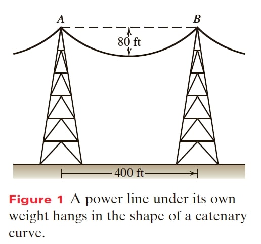
For the electrical power line depicted in Figure 1, the maximum design sag is restricted to 80 ft. Determine the length of the cable and the maximum tension assuming that the shape of the cable is parabolic. Compare your answers with those from Example 11.2.1 in which the cable was modeled as a catenary.
Learn more on how we answer questions.
Goal Find L and T_{max} using the parabolic approach, then compare the result with Example 11.2.1.
Given Information about the geometry and weight of the power line as well as a specific design constraint.
Assume The cable is inextensible.
Draw Figure 2 represents the location of the origin for either a catenary or a parabolic shape.
Formulate Equations and Solve In the parabolic method approach, the weight of the cable is modeled as a uniform weight per horizontal distance (ω) hanging from the cable, which we calculate by dividing the weight of the cable by the distance between the towers.
\omega =\frac{F_{cable}}{W}
where
F_{cable}=\mu L=(1 lb/ft)L
Equation (IV.5b) is independent of ω, so we can find the length L of the cable using x_{A}= −200 ft ,y_{A}=80 ft , x_{B}= 200 ft , and y_{B}= 80 ft:
L = – x_{A}\left[1+ \frac{2}{3}\left\lgroup \frac{y_{A}}{x_{A}} \right\rgroup^{2}- \frac{2}{5} \left\lgroup\frac{y_{A}}{x_{A}} \right\rgroup^{4} \right] + x_{B} \left[1+\frac{2}{3} \left\lgroup\frac{y_{A}}{x_{B}} \right\rgroup^{2}- \frac{2}{5} \left\lgroup\frac{y_{B}}{x_{B}} \right\rgroup^{4} \right]
=- \left(-200\right) \left[1+\frac{2}{3}\left\lgroup\frac{80 ft}{- 200 ft} \right\rgroup ^{2}- \frac{2}{5} \left\lgroup\frac{80 ft}{- 200 ft} \right\rgroup ^{4} \right] + 200 ft\left[1+\frac{2}{3}\left\lgroup\frac{80 ft}{ 200 ft} \right\rgroup ^{2}- \frac{2}{5} \left\lgroup\frac{80 ft}{ 200 ft} \right\rgroup ^{4}\right] \Rightarrow L=438.6 ft
Therefore
\omega =\frac{F_{cable}}{W} =\frac{(1 lb/ft)438.6 ft}{400 ft}= 1.096 lb/ft
Equation (11.3A) describes the parabolic shape of the hanging cable, which is constrained by the 80-ft sag and the 400-ft distance between the towers. We rearrange (11.3A) to solve for T_{O}:
T_{O}=\frac{\omega x^{2}}{2 y} \underbrace{= }_{x=200 ft,y=80 ft} \frac{1.096 lb/ft(200 ft)^{2}}{2(80 ft)} =274.1 lb
Using (11.4), we find T_{max} , which occurs at either of the towers:
T_{max}=\sqrt{\omega ^{2} x^{2} + T_{O}^{2}}=\sqrt{(1.096 lb/ft)^{2} (200 ft)^{2}+ (274.1 lb)^{2}} \Rightarrow T_{max}=351.0 lb
In Example 11.2.1 T_{max}= 342 lb and L = 440 ft. For this example (sag-to-span ratio y_{sag} /W = 80/400 = 0.2 ), the difference in the answers is not large. For larger sag-to-span ratios, the catenary approach will generate more accurate solutions than the parabolic approach for the self-weight loading case. As a general rule, the parabolic approach is only recommended for sag-to-span ratios of 0.1 or less.
