Known: A curved, solar absorber surface with a special coating is being cured by use of an infrared heater in a large room.
Find: Net rate of heat transfer to the absorber surface.
Schematic:
Assumptions:
1. Steady-state conditions exist.
2. Convection effects are negligible.
3. Absorber and heater surfaces are diffuse and gray and are characterized by uniform irradiation and radiosity.
4. The surrounding room is large and therefore behaves as a blackbody.
Analysis: The system may be viewed as a three-surface enclosure, with the third surface being the large surrounding room, which behaves as a blackbody. We are interested in obtaining the net rate of radiation transfer to surface 2. We solve the problem using both the radiation network and direct approaches.
Radiation Network Approach The radiation network is constructed by first identifying nodes associated with the radiosities of each surface, as shown in step 1 in the following schematic. Then each radiosity node is connected to each of the other radiosity nodes through the appropriate space resistance, as shown in step 2. We will treat the surroundings as having a large but unspecified area, which introduces difficulty in expressing the space resistances (A_{3}F_{31})^{-1} and (A_{3}F_{32})^{-1}. Fortunately, from the reciprocity relation (Equation 13.3), we can replace A_{3}F_{31} with A_{1}F_{13} and A_{3}F_{32} with A_{2}F_{23}, which are more readily obtained. The final step is to connect the blackbody emissive powers associated with the temperature of each surface to the radiosity nodes, using the appropriate form of the surface resistance.
A_{i}F_{ij} = A_{j}F_{ji} (13.3)


In this problem, the surface resistance associated with surface 3 is zero according to assumption 4; therefore, J_{3} = E_{b3} = σT_{3}^{4} = 459 W/m^{2}.
Summing currents at the J_{1} node yields
\frac{σT_{1}^{4} – J_{1}}{(1 – ε_{1})/ε_{1}A_{1}} = \frac{J_{1} – J_{2}}{1/A_{1}F_{12}} + \frac{J_{1} – σT_{3}^{4}}{1/A_{1}F_{13}} (1)
while summing the currents at the J_{2} node results in
\frac{σT_{2}^{4} – J_{2}}{(1 – ε_{2})/ε_{2}A_{2}} = \frac{J_{2} – J_{1}}{1/A_{1}F_{12}} + \frac{J_{2} – σT_{3}^{4}}{1/A_{2}F_{23}} (2)
The view factor F_{12} may be obtained by recognizing that F_{12} = F_{12'}, where A'_{2} is shown in the schematic as the rectangular base of the absorber surface. Then, from Figure 13.4 or Table 13.2, with Y/L = 10/1 = 10 and X/L = 1/1 = 1,
| TABLE 13.2 View Factors for Three-Dimensional Geometries [4] | |
| Geometry | Relation |
| Aligned Parallel Rectangles (Figure 13.4)
|
\overline{X} = X/L, \overline{Y} = Y/L\\ F_{ij} = \frac{2}{\pi \overline{X}\overline{Y}}\left\{\ln \left[\frac{(1 + \overline{X}^{2})(1 + \overline{Y}^{2})}{1 +\overline{X}^{2}+ \overline{Y}^{2}}\right]^{1/2} + \overline{X}(1 + \overline{Y}^{2})^{1/2} \tan^{-1}\frac{\overline{X}}{(1 + \overline{Y}^{2})^{1/2}} + \overline{Y}(1 + \overline{X}^{2})^{1/2} \tan^{-1}\frac{\overline{Y}}{(1 + \overline{X}^{2})^{1/2}} – \overline{X} \tan^{-1} \overline{X} – \overline{Y} \tan^{-1} \overline{Y}\right\} |
| Coaxial Parallel Disks (Figure 13.5)
|
R_{i} = r_{i}/L, R_{j} = r_{j}/L\\ S = 1 + \frac{1 + R^{2}_{j}}{R^{2}_{i}}\\ F_{ij} = \frac{1}{2} \left\{S – [S^{2} – 4(r_{j}/r_{i})^{2}]^{1/2}\right\} |
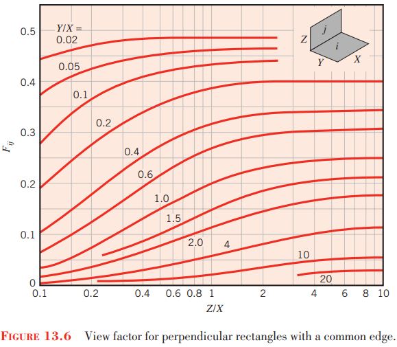
| Perpendicular Rectangles with a Common Edge (Figure 13.6)
|
H = Z/X, W = Y/X\\ F_{ij} = \frac{1}{\pi W} \left(W\tan^{-1} \frac{1}{W} + H \tan^{-1} \frac{1}{H} – (H^{2} + W^{2})^{1/2} \tan^{-1} \frac{1}{(H^{2} + W^{2})^{1/2}} + \frac{1}{4}\ln \left\{\frac{(1 + W^{2})(1 + H^{2})}{1 + W^{2} + H^{2}}\left[\frac{W^{2}(1 + W^{2} + H^{2})}{(1 + W^{2})(W^{2} + H^{2})}\right]^{W^{2}} \times \left[\frac{H^{2}(1 + H^{2} + W^{2})}{(1 + H^{2})(H^{2} + W^{2})}\right]^{H^{2}}\right\} \right) |


F_{12} = 0.39
From the summation rule, and recognizing that F_{11} = 0, it also follows that
F_{13} = 1 – F_{12} = 1 – 0.39 = 0.61
The last needed view factor is F_{23}. We recognize that, since radiation propagating from surface 2 to surface 3 must pass through the hypothetical surface A'_{2},
A_{2}F_{23} = A'_{2}F_{2'3}
and from symmetry F_{2'3} = F_{13}. Thus
F_{23} = \frac{A'_{2}}{A_{2}}F_{13} = \frac{10 m^{2}}{15 m^{2}} × 0.61 = 0.41
We may now solve Equations 1 and 2 for J_{1} and J_{2}. Recognizing that E_{b1} = σT_{1}^{4} = 56,700 W/m^{2} and canceling the area A_{1}, we can express Equation 1 as
\frac{56,700 – J_{1}}{(1 – 0.9)/0.9} = \frac{J_{1} – J_{2}}{1/0.39} + \frac{J_{1} – 459}{1/0.61}
or
-10J_{1} + 0.39J_{2} = -510,582 (3)
Noting that E_{b2} = σT_{2}^{4} = 7348 W/m^{2} and dividing by the area A_{2}, we can express Equation 2 as
\frac{7348 – J_{2}}{(1 – 0.5)/0.5} = \frac{J_{2} – J_{1}}{15 m^{2}/(10 m^{2} × 0.39)} + \frac{J_{2} – 459}{1/0.41}
or
0.26J_{1} – 1.67J_{2} = -7536 (4)
Solving Equations 3 and 4 simultaneously yields J_{2} = 12,487 W/m^{2}.
An expression for the net rate of heat transfer from the absorber surface, q_{2}, may be written upon inspection of the radiation network and is
q_{2} = \frac{σT_{2}^{4} – J_{2}}{(1 – ε_{2})/ε_{2}A_{2}}
resulting in
q_{2} = \frac{(7348 – 12,487)W/m^{2}}{(1 – 0.5)/(0.5 × 15 m^{2})} = -77.1 kW
Hence, the net heat transfer rate to the absorber is q_{net} = -q_{2} = 77.1 kW.
Direct Approach Using the direct approach, we write Equation 13.21 for each of the three surfaces. We use reciprocity to rewrite the space resistances in terms of the known view factors from above and to eliminate A_{3}.
\frac{E_{bi} – J_{i}}{(1 – ε_{i})/ε_{i}A_{i}} = \sum\limits_{j=1}^{N} \frac{J_{i} – J_{j}}{(A_{i}F_{ij})^{-1}} (13.21)
Surface 1
\frac{σT_{1}^{4} – J_{1}}{(1 – ε_{1})/ε_{1}A_{1}} = \frac{J_{1} – J_{2}}{1/A_{1}F_{12}} + \frac{J_{1} – J_{3}}{1/A_{1}F_{13}} (5)
Surface 2
\frac{σT_{2}^{4} – J_{2}}{(1 – ε_{2})/ε_{2}A_{2}} = \frac{J_{2} – J_{1}}{1/A_{2}F_{21}} + \frac{J_{2} – J_{3}}{1/A_{2}F_{23}} = \frac{J_{2} – J_{1}}{1/A_{1}F_{12}} + \frac{J_{2} – J_{3}}{1/A_{2}F_{23}} (6)
Surface 3
\frac{σT_{3}^{4} – J_{3}}{(1 – ε_{3})/ε_{3}A_{3}} = \frac{J_{3} – J_{1}}{1/A_{3}F_{31}} + \frac{J_{3} – J_{2}}{1/A_{3}F_{32}} = \frac{J_{3} – J_{1}}{1/A_{1}F_{13}} + \frac{J_{3} – J_{2}}{1/A_{2}F_{23}} (7)
Substituting values of the areas, temperatures, emissivities, and view factors into Equations 5 through 7 and solving them simultaneously, we obtain J_{1} = 51,541 W/m^{2}, J_{2} = 12,487 W/m^{2}, and J_{3} = 459 W/m^{2}. Equation 13.19 may then be written for surface 2 as
q_{i} = \frac{E_{bi} – J_{i}}{(1 – ε_{i})/ε_{i}A_{i}} (13.19)
q_{2} = \frac{σT_{2}^{4} – J_{2}}{(1 – ε_{2})/ε_{2}A_{2}}
This expression is identical to the expression that was developed using the radiation network. Hence, q_{2} = -77.1 kW.
Comments:
1. In order to solve Equations 5 through 7 simultaneously, we must first multiply both sides of Equation 7 by (1 – ε_{3})/ε_{3}A_{3} = 0 to avoid division by zero, resulting in the simplified form of Equation 7, which is J_{3} = σT_{3}^{4}.
2. If we substitute J_{3} = σT_{3}^{4} into Equations 5 and 6, it is evident that Equations 5 and 6 are identical to Equations 1 and 2, respectively.
3. The direct approach is recommended for problems involving N ≥ 4 surfaces, since radiation networks become quite complex as the number of surfaces increases.
4. As will be seen in Section 13.4, the radiation network approach is particularly useful when thermal energy is transferred to or from surfaces by additional means, that is, by conduction and/or convection. In these multimode heat transfer situations, the additional energy delivered to or taken from the surface can be represented by additional current into or out of a node.
5. Recognize the utility of using a hypothetical surface (A'_{2}) to simplify the evaluation of view factors.
6. We could have approached the solution in a slightly different manner. Radiation leaving surface 1 must pass through the openings (hypothetical surface 3′) in order to reach the surroundings. Thus, we can write.
F_{13} = F_{13'}
A_{1}F_{13} = A_{1}F_{13'} = A'_{3}F_{3'1}
A similar relationship can be written for exchange between surface 2 and the surroundings, that is, A_{2}F_{23} = A'_{3}F_{3'2}. Thus, the space resistances which connect to radiosity node 3 in the radiation network above can be replaced by space resistances pertaining to surface 3′. The resistance network would be unchanged, and the space resistances would have the same values as those determined in the foregoing solution. However, it may be more convenient to calculate the view factors by utilizing the hypothetical surfaces 3′. With the surface resistance for surface 3 equal to zero, we see that openings of enclosures that exchange radiation with large surroundings may be treated as hypothetical, nonreflecting black surfaces (ε_{3} = 1) whose temperature is equal to that of the surroundings (T_{3} = T_{sur}).
7. The heater and absorber surfaces would not be characterized by uniform irradiation or radiosity. The calculated heat rate could be checked by dividing the heater and absorber into subsurfaces, and repeating the analysis.