Question 9.CS.5: Linear algebraic equations can arise when modeling distribut...
Linear algebraic equations can arise when modeling distributed systems. For example, Fig. 9.7 shows a long, thin rod positioned between two walls that are held at constant temperatures. Heat flows through the rod as well as between the rod and the surrounding air. For the steady-state case, a differential equation based on heat conservation can be written for such a system as
\frac{d^2 T}{d x^2}+h^{\prime}\left(T_a-T\right)=0 (9.24)
where T = temperature (°C), x = distance along the rod (m), h′ = a heat transfer coefficient between the rod and the surrounding air (m−2), and T_a = the air temperature (°C).
Given values for the parameters, forcing functions, and boundary conditions, calculus can be used to develop an analytical solution. For example, if h′ = 0.01, T_a = 20, T(0) = 40, and T(10) = 200, the solution is
T=73.4523 e^{a .1 x}-53.4523 e^{-0.1 x}+20 (9.25)
Although it provided a solution here, calculus does not work for all such problems. In such instances, numerical methods provide a valuable alternative. In this case study, we will use finite differences to transform this differential equation into a tridiagonal system of linear algebraic equations which can be readily solved using the numerical methods described in this chapter.

Learn more on how do we answer questions.
Equation (9.24) can be transformed into a set of linear algebraic equations by conceptualizing the rod as consisting of a series of nodes. For example, the rod in Fig. 9.7 is divided into six equispaced nodes. Since the rod has a length of 10, the spacing between nodes is Δx = 2.
Calculus was necessary to solve Eq. (9.24) because it includes a second derivative.
As we learned in Sec. 4.3.4, finite-difference approximations provide a means to transform derivatives into algebraic form. For example, the second derivative at each node can be approximated as
where T_i designates the temperature at node i. This approximation can be substituted into Eq. (9.24) to give
\frac{T_{i+1}-2 T_i+T_{i-1}}{\Delta x^2}+h^{\prime}\left(T_a-T_i\right)=0Collecting terms and substituting the parameters gives
-T_{i-1}+2.04 T_i-T_{i+1}=0.8 (9.26)
Thus, Eq. (9.24) has been transformed from a differential equation into an algebraic equation. Equation (9.26) can now be applied to each of the interior nodes:
\begin{array}{l}-T_0+2.04 T_1-T_2=0.8 \\-T_1+2.04 T_2-T_3=0.8 \\-T_2+2.04 T_3-T_4=0.8 \\-T_3+2.04 T_4-T_5=0.8\end{array} (9.27)
The values of the fixed end temperatures, T_0 = 40 \text{ and } T_5 = 200, can be substituted and moved to the right-hand side. The results are four equations with four unknowns expressed in matrix form as
\left[\begin{array}{cccc}2.04 & -1 & 0 & 0 \\-1 & 2.04 & -1 & 0 \\0 & -1 & 2.04 & -1 \\0 & 0 & -1 & 2.04\end{array}\right]\left\{\begin{array}{l}T_1 \\T_2 \\T_3 \\T_4\end{array}\right\}=\left\{\begin{array}{r}40.8 \\0.8 \\0.8 \\200.8\end{array}\right\} (9.28)
So our original differential equation has been converted into an equivalent system of linear algebraic equations. Consequently, we can use the techniques described in this chapter to solve for the temperatures. For example, using MATLAB
>> A = [2.04 −1 0 0
−1 2.04 −1 0
0 −1 2.04 −1
0 0 −1 2.04];
>> b = [40.8 0.8 0.8 200.8]';
>> T = (A\b)'
T =
65.9698 93.7785 124.5382 159.4795
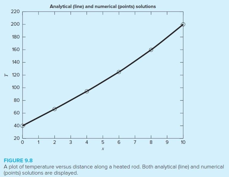
A plot can also be developed comparing these results with the analytical solution obtained with Eq. (9.25),
>> T = [40 T 200];
>> x = [0:2:10];
>> xanal = [0:10];
>> TT = @(x) 73.4523*exp(0.1*x)−53.4523* ...
exp(−0.1*x)+20;
>> Tanal = TT(xanal);
>> plot(x,T,'o',xanal,Tanal)
As in Fig. 9.8, the numerical results are quite close to those obtained with calculus.
In addition to being a linear system, notice that Eq. (9.28) is also tridiagonal. We can use an efficient solution scheme like the M-file in Fig. 9.6 to obtain the solution:
>> e = [0 −1 −1 −1];
>> f = [2.04 2.04 2.04 2.04];
>> g = [−1 −1 −1 0];
>> r = [40.8 0.8 0.8 200.8];
>> Tridiag(e,f,g,r)
ans =
65.9698 93.7785 124.5382 159.4795
The system is tridiagonal because each node depends only on its adjacent nodes.
Because we numbered the nodes sequentially, the resulting equations are tridiagonal. Such cases often occur when solving differential equations based on conservation laws.