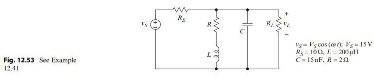
Question 12.41: Refer to Fig. 12.53. Express the average power dissipated in...

We first obtain the Thévenin equivalent for the circuit to the left of the load R_L. Kirchhoff’s current law gives

\begin{aligned} &\tilde{V}_T\left(\frac{1}{R_S}+\frac{1}{R+j \omega L}+j \omega C\right)=\frac{V_S}{R_S} \\\\ &\Rightarrow \tilde{V}_T=\frac{(R+j \omega L) V_S}{R_S+R-R_S L C \omega^2+j \omega\left(L+R_S R C\right)} \end{aligned}

where \nu_S is the phase reference and \tilde{V}_T is the open-circuit (Thévenin equivalent) voltage. The short-circuit (Norton equivalent) current is given by

  \tilde{I}_N=\frac{V_S}{R_S},

so the Thévenin equivalent impedance is given by

Z_T=\frac{\tilde{V}_T}{\tilde{I}_N}=\frac{(R+j \omega L) R_S}{R_S+R-R_S L C \omega^2+j \omega\left(L+R_S R C\right)},

 where f  is the frequency of the source and  \omega=2 \pi f . The rms amplitude of the voltage across a load  R_L is given by

V_{L \mathrm{rms}}=\left|\frac{V_S R_L}{\sqrt{2}\left(Z_T+R_L\right)}\right|

 and the power dissipated by the load is given by

P_L=\frac{V_{L \mathrm{rms}^2}}{R_L} .

Figure  12.54 shows a (computer-generated) graph of the power dissipated versus the load resistance. The load resistance that draws maximum power is approximately  R_L=10  \Omega . To see if this result is reasonable, we calculate the Thévenin impedance for  f=30  \mathrm{kHz} . We obtain  Z_T=(9.35+j 2.18)  \Omega , so we might expect maximum power transfer for a load in the neighborhood of  10  \Omega . We also expect the power dissipated to approach zero for  R_L \rightarrow 0 , in which case the load voltage approaches zero, and for  R_L \rightarrow \infty , in which case the load current approaches zero. The graph in Fig.  12.54  is consistent with these expectations.

Figure  12.55 shows a computer-generated graph of the power dissipated in the load  R_L=10  \Omega versus frequency. Maximum power is dissipated for frequencies near 100  \mathrm{kHz} . This is not surprising, because the magnitude of the impedance of the parallel  RLC  branch at that frequency is  678  \Omega , which is much larger than both the source resistance and the load resistance. Thus the parallel  RLC  branch draws very little current for frequencies near  100  \mathrm{kHz} . For frequencies approaching zero, the impedance of the parallel  RLC  branch approaches  R=2  \Omega , so the load voltage approaches

   V_{L \mathrm{rms}}(f \rightarrow 0)=\frac{R \| R_L}{R_S+R \| R_L} \frac{V_S}{\sqrt{2}} \cong 1.52 \mathrm{~V},

and the power dissipated approaches

   P_L(f \rightarrow 0)=\frac{V_{L \mathrm{rms}}^2}{R_L} \cong 230 \mathrm{~mW} .  

For frequencies much larger than  100   \mathrm{kHz} , the impedance of the parallel  RLC branch approaches the impedance of the capacitor,

which in turn approaches zero, so the parallel  RLC  branch shunts virtually all of the current to ground and the power dissipated by the load approaches zero. The graph in Fig.  12.55  is consistent with these observations.

This example illustrates using a Thévenin equivalent to simplify studying load power (or current or voltage) as a function of the load impedance and source frequency. Using the Thévenin equivalent means we must solve equations obtained from (e.g.) Kirchhoff’s current law only once. Thereafter, the circuit is simply a voltage divider, and subsequent analysis is relatively simple.