Question 11.26: Solve the spinning top problem of Example 11.15 numerically,...

We will use Eq. (11.72) (the Euler equations) to compute the body frame angular velocity derivatives:

\frac{ d \omega_x}{ d t}=\frac{M_x}{A}-\frac{C-B}{A} \omega_y \omega_z

\frac{ d \omega_y}{ dt }=\frac{M_y}{B}-\frac{A-C}{B} \omega_z \omega_x                    (a)

\frac{ d \omega_z}{ d t}=\frac{M_z}{C}-\frac{B-A}{C} \omega_x \omega_y

\left. M _{\text {net }}=\dot{ H }\right)_{ rel }+ \omega \times H                  (11.72a)

\left.M_x\right)_{\text {net }}=A \dot{\omega}_x+(C-B) \omega_y \omega_z

\left.M_y\right)_{\text {net }}=B \dot{\omega}_y+(A-C) \omega_z \omega_x                     (11.72b)

\left.M_z\right)_{ net }=C \dot{\omega}_z+(B-A) \omega_x \omega_y

These require that the moving xyz axes are all rigidly attached to the top. In Example 11.15 only the x axis was fixed to the top along its spin axis; the y and z axes did not rotate with the top.

The moments in Eq. (a) must be expressed in components along the body-fixed axes. From Fig. 11.19, the moment of
the weight vector about O is

M =d \hat{ k } \times(-m g \hat{ K })=-m g d(\hat{ k } \times \hat{ K })                      (b)

where, recalling Eq. (4.18)3

\hat{ k }=Q_{31} \hat{ I }+Q_{32} \hat{ J }+Q_{33} \hat{ K }                        (c)

The Qs are the time-dependent components of the direction cosine matrix [ Q ]_{X x} in Eq. (11.157). Carrying out the cross product in Eq. (b) yields the components of M along the XYZ axes of the fixed space frame,

[ Q ]_{X x}=\left[\begin{array}{ccc}q_1^2-q_2^2-q_3^2+q_4^2 & 2\left(q_1 q_2+q_3 q_4\right) & 2\left(q_1 q_3-q_2 q_4\right) \\2\left(q_2 q_1-q_3 q_4\right) & -q_1^2+q_2^2-q_3^2+q_4^2 & 2\left(q_2 q_3+q_1 q_4\right) \\2\left(q_3 q_1+q_2 q_4\right) & 2\left(q_3 q_2-q_1 q_4\right) & -q_1^2-q_2^2+q_3^2+q_4^2\end{array}\right]                       (11.157)

\{ M \}_X=\left\{\begin{array}{c}-m g d Q_{32} \\m g d Q_{31} \\0\end{array}\right\}

To obtain the components of M in the body-fixed frame, we perform the transformation

\{ M \}_x=[ Q ]_{X_x}\{ M \}_X=\left[\begin{array}{lll}Q_{11} & Q_{12} & Q_{13} \\Q_{21} & Q_{22} & Q_{23} \\Q_{31} & Q_{32} & Q_{33}\end{array}\right]\left\{\begin{array}{c}-m g d Q_{32} \\m g d Q_{31} \\0\end{array}\right\}=m g d\left\{\begin{array}{c}Q_{12} Q_{31}-Q_{32} Q_{11} \\Q_{22} Q_{31}-Q_{32} Q_{21} \\0\end{array}\right\}                           (d)

It can be shown that (Problem 11.27)

Q_{12} Q_{31}-Q_{32} Q_{11}=Q_{23} \quad Q_{22} Q_{31}-Q_{32} Q_{21}=-Q_{13}

Therefore, at any instant the moments in Eq. (a) are

M_x=m g d Q_{23} \quad M_y=-m g d Q_{13} \quad M_z=0                         (e)

The MATLAB implementation of the following procedure is listed in Appendix D.51.
Step 1:
Specify the initial orientation of the xyz axes of the body frame, thereby defining the initial value of the direction cosine matrix [ Q ]_{X x}.

According to Fig. 11.19, the body z axis is the top’s spin axis, and we shall assume here that it initially lies in the global YZ plane, tilted 60° away from the Z axis, as it is in Example 11.15. Let the body x axis be initially aligned with the global X axis. The body y axis is then found from the cross product \hat{ j }=\hat{ k } \times \hat{ i }. Thus,

\hat{ k }=-\sin 60^{\circ} \hat{ J }+\cos 60^{\circ} \hat{ K }

\hat{ i }=\hat{ I }

\hat{ j }=\hat{ k } \times \hat{ i }=\cos 60^{\circ} \hat{ J }+\sin 60^{\circ} \hat{ K }

It follows that the direction cosine matrix relating XYZ to xyz at the start of the simulation is

\left[Q_0\right]_{X x}=\left[\begin{array}{ccc}1 & 0 & 0 \\0 & \cos 60^{\circ} & \sin 60^{\circ} \\0 & -\sin 60^{\circ} & \cos 60^{\circ}\end{array}\right]=\left[\begin{array}{ccc}1 & 0 & 0 \\0 & 1 / 2 & \sqrt{3} / 2 \\0 & -\sqrt{3} / 2 & 1 / 2\end{array}\right]                        (f)

Step 2:
Compute the initial quaternion \hat{ q }_0 using Algorithm 11.2. Substituting Eq. (f) into Eq. (11.150) yields

[ K ]=\left[\begin{array}{cccc}0 & 0 & 0 & 0.57735 \\0 & -0.33333 & 0 & 0 \\0 & 0 & -0.33333 & 0 \\0.57735 & 0 & 0 & 0.66667\end{array}\right]

\widetilde{q}^{-1}=\frac{\widehat{q}^*}{\|\widehat{q}\|^2}                  (11.150)

Rather than finding the dominant eigenvector by means of the power method, as we did in Example 11.23, we shall here use MATLAB’s eig function, which obtains all of the eigenpairs. The snippet of MATLAB code for doing so is:

Therefore, the initial value of the quaternion is

\widehat{ q }_0=\left\{\begin{array}{c}0.5 \\0 \\0 \\\hdashline 0.86603\end{array}\right\}                     (g)

Step 3:
Specify the initial values of the body frame components of angular velocity \omega _0=\left[\begin{array}{lll}\left.\omega_x\right)_0 & \left.\omega_y\right)_0 &\left.\omega_z\right)_0\end{array}\right]^T.

Recall that Eq. (11.115) relate these body frame angular velocities to the initial values of the top’s Euler angles and their rates,

\left.\left.\left.\omega_x\right)_0=\omega_p\right)_0 \sin \theta_0 \sin \psi_0+\omega_n\right)_0 \cos \psi_0

\left.\left.\left.\omega_y\right)_0=\omega_p\right)_0 \sin \theta_0 \cos \psi_0-\omega_n\right)_0 \sin \psi_0                              (h)

\left.\left.\left.\omega_z\right)_0=\omega_s\right)_0+\omega_p\right)_0 \cos \theta_0

The top is released from rest with a given tilt angle \theta_0 and spin rate \left.\omega_s\right)_0. According to Example 11.15,

\theta_0=60^{\circ}

\psi_0= 0

\left.\omega_s\right)_0=1000 rpm =104.72 rad / s                    (i)

\left.\omega_p\right)_0 = 51.93 rpm = 5.438 rad/s (low energy precession rate)

\left.\omega_n\right)_0 = 0

Substituting these into Eq. (h) we find

\omega_0=\left[\begin{array}{lll}0 & 4.7095 & 107.44\end{array}\right]^T  ( rad / s )                     (j)

Step 4:
Supply \omega _0 and \hat{ q }_0 as initial conditions to, say, the Runge–Kutta–Fehlberg 4(5) numerical integration procedure (Algorithm 1.3) to solve the system \{\dot{ y }\}=\{ f \}, where

\{ y \}=\left[\begin{array}{lllllll}\omega_x &\omega_y & \omega_z & q_1 & q_2 & q_3 & q_4\end{array}\right]^T                   (k)

\{ f \}=\left\lfloor d \omega_x / d t \quad d \omega_y / d t \quad d \omega_2 / d t \quad d q_1 / d t \quad d q_2 / d t \quad d q_3 / d t \quad d q_4 / d t\right\rfloor^T

thereby obtaining the angular velocity ω and quaternion \hat{ q } as functions of time. At each step of the numerical integration process:

(i) Use the current value of \hat{ q } to compute [ Q ]_{X x} from Algorithm 11.1.
(ii) Use the current value of [ Q ]_{X x} and ω to compute dω=dt from (a), (d), and (e).
(iii) Use the current value of \hat{ q } and ω to compute d \hat{ q }/dt from Eqs. (11.164).

\dot{\hat{ u }}=\frac{1}{2}[\hat{ u } \times \omega -\cot (\theta / 2) \hat{ u } \times(\hat{ u } \times \omega )]                      (11.164)

Step 5:
At each solution time:
(i) Use Algorithm 11.1 to compute the direction cosine matrix [ Q ]_{X x}.
(ii) Use Algorithm 4.3 to compute the Euler angles ϕ (precession), θ (nutation), and ψ(spin).
(iii) Use Eq. (11.116) to compute the Euler angle rates \dot{\phi}, \dot{\theta}, and \dot{\psi}.

\left\{\begin{array}{l}\omega_p \\\omega_n \\\omega_s\end{array}\right\}=\left[\begin{array}{ccc}\sin \psi / \sin \theta & \cos \psi / \sin \theta & 0 \\\cos \psi & -\sin \psi & 0 \\-\sin \psi / \tan \theta & -\cos \psi / \tan \theta & 1\end{array}\right]\left\{\begin{array}{l}\omega_x \\\omega_y \\\omega_z\end{array}\right\}                      (11.116a)

\omega_p=\dot{\phi}=\frac{1}{\sin \theta}\left(\omega_x \sin \psi+\omega_y \cos \psi\right)

\omega_n=\dot{\theta}=\omega_x \cos \psi-\omega_y \sin \psi                 (11.116b)

\omega_s=\dot{\psi}=-\frac{1}{\tan \theta}\left(\omega_x \sin \psi+\omega_y \cos \psi\right)+\omega_z

Step 6:
Plot the time histories of the Euler angles and their rates.
Fig. 11.34 shows the numerical solution for the precession, nutation, and spin angles as well as their rates as functions of time. We see that the constant precession rate (51.93 rpm) and spin rate (1000 rpm) are in agreement with Example 11.15, as is the nutation angle, which is fixed at 60°. The sawtooth appearance of the spin angle ψ(t) reflects the fact that it is confined to the range 0 to 360°.

Clearly , the solution of the steady-state spinning top problem by numerical integration yields no new insight into the top’s motion and may be deemed a waste of effort. However, suppose we solve the same problem, but release the top from rest with zero precession rate, so that instead of Eqs. (i), the initial conditions are

\theta_0=60^{\circ}

\psi_0= 0

\left.\omega_s\right)_0=1000 rpm =104.72 rad / s                    (l)

\left.\omega_p\right)_0 = 0

\left.\omega_n\right)_0 = 0

The initial orientation of the top is unchanged, so the initial quaternion \hat{ q }_0 remains as shown in Eq. (g). On the other hand, the initially zero precession rate yields a different initial angular velocity vector, namely,

\omega _0=\left\lfloor\begin{array}{lll}0 & 0 & 104.72\end{array}\right]^T( rad / s )                           (m)

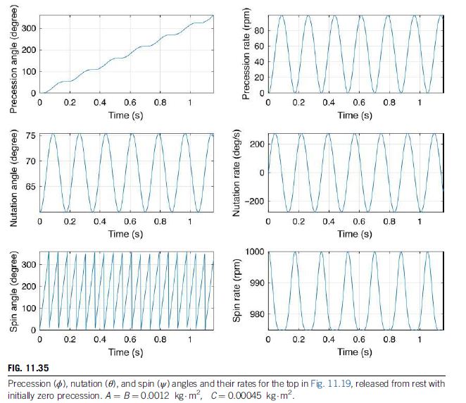
With only this change, the above numerical integration procedure yields the results shown in Fig. 11.35.

This is an example of unsteady precession, in which we see that the spin axis, instead of making a constant angle of 60° to the vertical, nutates between 60° and 75.4° at a rate of about 5.7 Hz, while the spin rate itself varies between 975 and 1000 rpm at the same frequency. The precession rate oscillates between 0 and 99.4 rpm, also at a frequency of 5.7 Hz, with an average rate of 51.9 rpm, which happens to be the steady-state precession rate (Fig. 11.34).

These numerical results can be compared with formulas from the classical analysis of tops in unsteady precession. For example, it can be shown (Greenwood, 1988) that the relationship between the minimum and maximum nutation angles is

\cos \theta_{\max }=\lambda-\sqrt{\lambda^2-2 \lambda \cos \theta_{\min }+1}

where \lambda=C^2 \omega_z^2 /(4 A m g d). For the data of this problem, λ = 1.887, so that

\cos \theta_{\max }=1.887-\sqrt{1.887^2-2 \cdot 1.887 \cdot \cos 60^{\circ}+1}=0.2518

\theta_{\max }=75.41^{\circ}

This is precisely what we observe for the nutation angle in Fig. 11.35. By the way, ωz remains constant at its initial value of 104.72 rad/s because the top is axisymmetric (A = B) and M_z= 0 (Eq. (e)_3) , so that dω_z/dt = 0 (Eq. (a)_3).