Question 10.4: Speed controls find wide application throughout industry and...

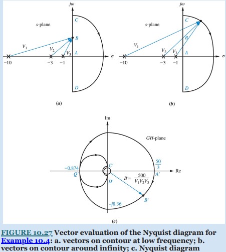
Conceptually, the Nyquist diagram is plotted by substituting the points of the contour shown in Figure 10.27(a) into G(s) = 500/[(s + 1)(s + 3)(s + 10)]. This process is equivalent to performing complex arithmetic using the vectors of G(s) drawn to the points of the contour as shown in Figure 10.27(a) and (b). Each pole and zero term of G(s) shown in Figure 10.26(b) is a vector in Figure 10.27(a) and (b). The resultant vector, R, found at any point along the contour is in general the product of the zero vectors divided by the product of the pole vectors [see Figure 10.27(c)]. Thus, the magnitude of the resultant is the product of the zero lengths divided by the product of the pole lengths, and the angle of the resultant is the sum of the zero angles minus the sum of the pole angles.

As we move in a clockwise direction around the contour from point A to point C in Figure 10.27(a), the resultant angle goes from 0° to −3 × 90° = −270°, or from A′ to C′ in Figure 10.27(c). Since the angles emanate from poles in the denominator of G(s), the rotation or increase in angle is really a decrease in angle of the function G(s); the poles gain 270° in a counterclockwise direction, which explains why the function loses 270°.

While the resultant moves from A′ to C′ in Figure 10.27(c), its magnitude changes as the product of the zero lengths divided by the product of the pole lengths. Thus, the resultant goes from a finite value at zero frequency [at point A of Figure 10.27(a), there are three finite pole lengths] to zero magnitude at infinite frequency at point C [at point C of Figure 10.27(a), there are three infinite pole lengths].

The mapping from point A to point C can also be explained analytically. From A to C, the collection of points along the contour is imaginary. Hence, from A to C, G(s) = G(jω), or from Figure 10.26(b),

G(jω) = \frac{500}{(s  +  1)  (s  +  3)  (s  +  10)} \mid _{s\rightarrow jω } = \frac{500}{(− 14ω²  +  30)  +  j  (43ω  −  ω³) }                       (10.40)

Multiplying the numerator and denominator by the complex conjugate of the denominator, we obtain

G(jω) = 500 \frac{(− 14ω²  +  30)  −  j (43ω  −  ω³)}{(− 14ω²  +  30)²  +  (43ω  −  ω³)²}       (10.41)

At zero frequency, G(jω) = 500/30 = 50/3. Thus, the Nyquist diagram starts at 50/3, at an angle of 0°. As ω increases, the real part remains positive and the imaginary part remains negative. At ω = \sqrt{30/14} , the real part becomes negative. At ω = \sqrt{43} , the Nyquist diagram crosses the negative real axis, since the imaginary term goes to zero. The real value at the axis crossing, point Q′ in Figure 10.27(c), found by substituting into Eq. (10.41), is −0.874. Continuing toward ω = ∞, the real part is negative, and the imaginary part is positive. At infinite frequency G(jω) ≈ j500/ω³, or approximately zero at 90°.

Around the infinite semicircle from point C to point D shown in Figure 10.27(b), the vectors rotate clockwise, each by 180°. Hence, the resultant undergoes a counterclockwise rotation of 3 × 180°, starting at point C′ and ending at point D′ of Figure 10.27(c). Analytically, we can see this by assuming that around the infinite semicircle, the vectors originate approximately at the origin and have infinite length. For any point on the s-plane, the value of G(s) can be found by representing each complex number in polar form, as follows:

G(s) = \frac{500}{ (R_{-1}  e^{jθ−1} )  (R_{-3}  e^{jθ−3} )  (R_{-10}  e^{jθ−10} )}                   (10.42)

where R_{-i} is the magnitude of the complex number (s + i), and θ_{-i} is the angle of the complex number (s + i). Around the infinite semicircle, all R_{-i} are infinite, and we can use our assumption to approximate the angles as if the vectors originated at the origin. Thus, around the infinite semicircle,

G(s) = \frac{500}{ \infty ∠ (θ_{-1}  +  θ_{-3}  +  θ_{-10}) } = 0 ∠  −  (θ_{-1}  +  θ_{-3}  +  θ_{-10})             (10.43)

At point C in Figure 10.27(b), the angles are all 90°. Hence, the resultant is 0∠ −270°, shown as point C′ in Figure 10.27(c). Similarly, at point D, G(s) = 0∠ + 270° and maps into point D′. You can select intermediate points to verify the spiral whose radius vector approaches zero at the origin, as shown in Figure 10.27(c).

The negative imaginary axis can be mapped by realizing that the real part of G(jω)H(jω) is always an even function, whereas the imaginary part of G(jω)H(jω) is an odd function. That is, the real part will not change sign when negative values of ω are used, whereas the imaginary part will change sign. Thus, the mapping of the negative imaginary axis is a mirror image of the mapping of the positive imaginary axis. The mapping of the section of the contour from points D to A is drawn as a mirror image about the real axis of the mapping of points A to C.