Question 4.4: Streamlines in the xy-Plane—An Analytical Solution For the s...
Streamlines in the xy-Plane—An Analytical Solution
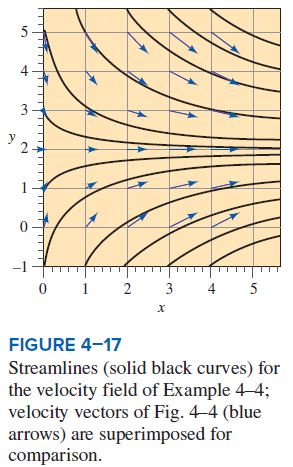
For the steady, incompressible, two-dimensional velocity field of Example 4–1, plot several streamlines in the right half of the flow (x > 0) and compare to the velocity vectors plotted in Fig. 4–4.

Learn more on how we answer questions.
An analytical expression for streamlines is to be generated and plotted in the upper-right quadrant.
Assumptions 1 The flow is steady and incompressible. 2 The flow is two-dimensional, implying no z-component of velocity and no variation of u or 𝜐 with z.
Analysis Equation 4–16 is applicable here; thus, along a streamline,
Streamline in the xy-plane: \left(\frac{dy}{dx} \right)_{along a streamline} = \frac{\upsilon }{u} (4–16)
\frac{dy}{dx} = \frac{\upsilon }{u} = \frac{1.5 – 0.8y}{0.5 + 0.8x}
We solve this differential equation by separation of variables:
\frac{dy}{1.5 – 0.8y} = \frac{dx}{0.5 + 0.8x} \rightarrow \int{\frac{dy}{1.5 – 0.8y} } = \int{\frac{dx}{0.5 + 0.8x} }
After some algebra, we solve for y as a function of x along a streamline,
y = \frac{C}{0.8(0.5 + 0.8x)} + 1.875
where C is a constant of integration that can be set to various values in order to plot the streamlines. Several streamlines of the given flow field are shown in Fig. 4–17.
Discussion The velocity vectors of Fig. 4–4 are superimposed on the streamlines of Fig. 4–17; the agreement is excellent in the sense that the velocity vectors point everywhere tangent to the streamlines. Note that speed cannot be determined directly from the streamlines alone.