The t -coordinates are suitably scaled to use the orthogonal polynomials found in Example 5 of Section 6.7:

The calculations involve only these vectors, not the specific formulas for the orthogonal polynomials. The best approximation to the data by polynomials in P _{2} is the orthogonal projection given by
\hat{p}=\frac{\left\langle g, p_{0}\right\rangle}{\left\langle p_{0}, p_{0}\right\rangle} p_{0}+\frac{\left\langle g, p_{1}\right\rangle}{\left\langle p_{1}, p_{1}\right\rangle} p_{1}+\frac{\left\langle g, p_{2}\right\rangle}{\left\langle p_{2}, p_{2}\right\rangle} p_{2}.
=\frac{20}{5} p_{0}-\frac{1}{10} p_{1}-\frac{7}{14} p_{2}.
and
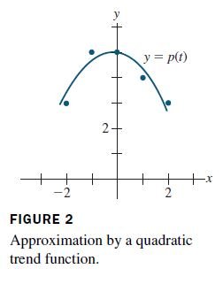
\hat{p}(t)=4-.1 t-.5\left(t^{2}-2\right) (3).
Since the coefficient of p_{2} is not extremely small, it would be reasonable to conclude that the trend is at least quadratic. This is confirmed by the graph in Figure 2.