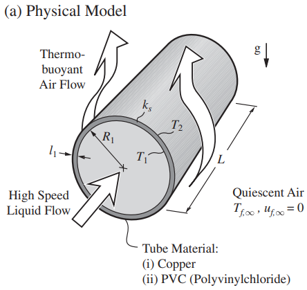
(a) The thermal circuit diagram is shown in Figure (b).
(b) The heat flowing through the composite layers is
Q_{k,1-2}=\frac{T_{1}-T_{2}}{R_{k,1-2}}
=\left\langle Q_{ku}\right\rangle _{D}=\frac{T_{2}-T_{f,\infty }}{\left\langle R_{ku}\right\rangle _{D}}
=\frac{T_{1}-T_{f,\infty }}{R_{k1-2}+\left\langle R_{ku}\right\rangle _{D}} \equiv \frac{T_{1}-T_{f,\infty }}{R_{\sum }} ,D=2(R_{1}+l_{1})
(c) The conduction resistance is found from Table, i.e.,
R_{k,1-2}=\frac{lnR_{2}/R_{1}}{2\pi Lk_{s}} =\frac{ln(R_{1}-R_{2})/R_{1}}{2\pi Lk_{s}}
The resistance \left\langle R_{ku}\right\rangle _{D} is related to \left\langle Nu\right\rangle _{D} through \left\langle Q_{ku}\right\rangle _{L( or D)}=\frac{T_{s}-T_{f,\infty }}{\left\langle R_{ku}\right\rangle_{L(or D)} } =A_{ku}\frac{k_{f}}{L(or D)}\left\langle Nu\right\rangle _{L(or D)}(T_{s}-T_{f,\infty }) ,Re_{L(or D)}=\frac{u_{f,\infty }L(or D)}{v_{f}} , i.e.,
\left\langle R_{ku}\right\rangle _{D}=\frac{D}{A_{ku}\left\langle Nu\right\rangle_{D}k_{f} } , A_{ku}=\pi DL
Now \left\langle Nu\right\rangle _{D} is given by the correlation in Table as
\left\langle Nu\right\rangle _{D}=(\left\langle Nu_{D,l}\right\rangle ^{3.3}+\left\langle Nu_{D.t}\right\rangle ^{3.3})^{1/33}
where Nu_{D,l} and N_{uD,t} are listed in Table and are related to the Rayleigh number
Ra_{D}=\frac{g\beta _{f}(T_{2}-T_{f,\infty })D^{3}}{v_{f}\alpha _{f}}
Here we note that \left\langle R_{ku}\right\rangle _{D}, through \left\langle Nu\right\rangle _{D}, depends on T_{2}, which is not known. We need to determine T_{2} and \left\langle R_{ku}\right\rangle _{D} simultaneously. For this we write \left\langle R_{ku}\right\rangle _{D}=\left\langle R_{ku}\right\rangle _{D}(T_{2}) and from the above heat flow rate equation, we rewrite
\frac{T_{1}-T_{2}}{R_{k,1-2}} =\frac{T_{1}-T_{f,\infty }}{R_{k,1-2}+\left\langle R_{ku}\right\rangle _{D}(T_{2})}
and then solve this for T_{2}. This is a nonlinear algebraic equation and is solvable by hand (through iteration) or by using a software.
We now write the expressions for \left\langle Nu_{D,l}\right\rangle and \left\langle Nu_{D,t}\right\rangle from Table, i.e.,
\left\langle Nu_{D,l}\right\rangle =\frac{1.6}{ln[1 + 1.6/(0.772a_{1}Ra^{1/4}_{D} )] }
\left\langle Nu_{D,t}\right\rangle =\frac{0.13Pr^{0.22}}{(1 + 0.61Pr^{0.81})^{ 0.42} } Ra^{1/3}_{D}
a_{1}=\frac{4}{3}\frac{0.503}{[1 + (0.492/Pr)^{9/16}]^{4/9}}
For the properties for air at T = 350 K, from Table, we have
Pr = 0.69
k_{f} = 0.0300 W/m-K
ν_{f} = 2.030 × 10^{−5} m^{2}/s
α_{f} = 2.944 × 10^{−5} m^{2}/s.
Also
\beta =\frac{1}{T}=\frac{1}{350(K)}
g = 9.807 m/s^{2}
A_{ku} = π(R_{1} + l_{1})L = π(0.15 + 0.001)(m) × 0.5(m) = 0.2512 m^{2}
D = 2(R_{1} + l_{1}) = 2(0.15 + 0.01)(m) = 0.32 m.
Then
Ra_{D}=\frac{9.8(m/s^{2}) × 2.857 × 10^{−3} (1/K) × (T_{2} − 293.16)(K) × (0.32)^{3} (m^{3}) }{2.030 × 10^{−5} (m^{2}/s) × 2.944 × 10^{−5} (m^{2}/s)}
a_{1} = 0.5132.
Now solving for T_{2}, we find
(i) copper : T_{2} = 353.14 K = 79.99^{\circ } C
(ii) PVC : T_{2} = 345.72 K = 72.576^{\circ }C.
The two surface-convection resistances are
(i) copper : Ra_{D} = 9.216 × 10^{7} , \left\langle Nu\right\rangle _{D} = 53.12
\left\langle R_{ku}\right\rangle _{D}(T_{2} = 353.14 K) = 0.3996^{\circ} C/W
(ii) PVC : Ra_{D} = 7.667 × 10^{7} , \left\langle Nu\right\rangle _{D} = 51.07
\left\langle R_{ku}\right\rangle _{D}(T_{2} = 345.72 K) = 0.4157^{\circ} C/W,
and the two conduction resistances are
(i) copper : R_{k,1-2} = 5.177 × 10^{−5 \circ} C/W
(ii) PVC : R_{k,1-2} = 0.05872^{\circ} C/W.
(d) From Bi_{L or D}=N_{ku,s}=\frac{R_{k,s}}{\left\langle R_{ku}\right\rangle _{L or D}} , the two Biot numbers are
Bi_{D}(copper) =Bi_{D}=\frac{R_{k,1-2}}{\left\langle R_{ku}\right\rangle _{D}} =\frac{5.177 × 10^{−5\circ } C/W}{0.3996^{\circ }C/W} = 1.296 × 10^{−4} < 0.1 substrate temperature drop is negligible
Bi_{D}(PVC) =\frac{0.05872 } {0.4157} = 0.1413 > 0.1 substrate temperature drop is significant.